
Summary, created by Matthias Meyer. Note there might be errors!
Some parts are also available on the following webpage.
To understand the topic of signal processing, one must be familiar with the following topics:
The derivation of Euler’s formula can be found in the following video. and the following: This formula allows us to describe a signal in a very easy way.

Note that the convolution has an identity element which is the δ(t) function, which’s integral is one.
Says that the energy in the time domain is the same as the energy in the frequency domain. Furthermore, it allows to see how the energy is distributed over different frequencies.


LTI means linear and time invariant. Which says that a linear combination of inputs generates the same linear combination of outputs and when I input a signal a little bit later into my system, I get the same output as if I would have entered the signal earlier. ⇒ no new frequencies can be produced and when the input is band limited also the output must be band limited.


A causal system is one that at a specific time, the output is only a function of the input at that time or before (but never after) Example of Casula systems:


Example of a not casual system


The value at the origin of the autocorrelation is equal to the energy of the signal. The energy spectral density is given by the following formula (see also parsevals theorem there is also the factor2π):

Note that the energy spectral density can also be calculated with the autocorrelation, as can be seen below:


When we talk about a periodic signal, we talk about the power spectral density. It has a discrete power spectrum density.

In a real valued signal there is redundant information in the negative-frequency part of the signal spectrum. Due to that, one can mask out the negative frequencies with the following formula:

As a result, one gets then the so-called analytic signal which lacks the symmetry properties in the Fourier transform and is therefore complex. ε(f) is the Heaviside step function. To get the analytic signal one can use the Hilbert transform, which is the convolution of x(t) with h(t) =  . See the formula below:

The Hilbert transforms frequency response can be found below, which is also called the hilbert filter.

The resulting analytic signal in the frequency domain is then the following:

Let x(t) be a band limited signal whose spectrum X(f) is limited to -f0 ≤ f ≤ f0
Compute the Hilbert transform of the band-pass signal
![˜x(t) = A(t)cos (2 πf0t + ϕ (t))
= A(t)[cos(2πf0t) cos(ϕ (t)) - sin(2πf0t) sin(ϕ(t))]
= A(t)cos(ϕ(t))cos (2 πf0t) - A (t)sin (ϕ(t)) sin (2πf0f )](main2_for_html24x.svg)
For a bandpass signal Equation 1 applys.
| (1) |
Therefore, the Hilbert transform is

Due to Ptolemy’s identities, the sum and difference formulas for sine and cosine, which can be found in Equation 2.
| (2) |
Compute the amplitude envelope of the signal x(t)
The analytic signal xa(t) of x(t) is

And the amplitude envelope is

Cascaded integrator-comb (CIC) digital filters are computationally-efficient implementations of narrowband lowpass filters, and are often embedded in hardware implementations of decimation, interpolation, and delta-sigma converter filtering.
An example can be found in Figure 12, where one sees it’s low pass filter behaviour. As the name describes, a CIC filter is a cascade of an integrator ( ) and a comp(1 - z-M) filter. The integrator is needed to cancel out the fist zero pole. The main advantage of this filter is described below (low computational effort) as well as the main disadvantage (nonlinearity).
CIC filters are well-suited for anti-aliasing filtering prior to decimation (sample rate reduction), as shown in Figure 3(a); and for anti-imaging filtering for interpolated signals (sample rate increase) as in Figure 3(b). Both applications are associated with very high-data rate filtering such as hardware quadrature modulation and demodulation in modern wireless systems, and delta-sigma A/D and D/A converters.
Because their frequency magnitude responses are sin(x)/x-like, CIC filters are typically followed, or preceded, by linear-phase lowpass tapped-delay line finite impulse response (FIR) filters whose tasks are to compensate for the CIC filter’s non-flat passband.
The Figure 3 cascaded-filter architectures have valuable benefits. For example:
CIC filters originate from the notion of a recursive running sum filter, which is itself an efficient form of a nonrecursive moving averager. Recall the standard D-point moving-average process in Figure 4(a). There we see that D-1 summations (plus one multiply by 1/D) are necessary to compute the averager’s y(n) output sequence.
The D-point moving-average filter’s time-domain output is expressed as
| (3) |
where n is our time-domain index. The z-domain expression for this moving averager’s output is
| (4) |
while its z-domain HMA(z) transfer function is
| (5) |
We provide these equations not to make things complicated, but because they’re useful. Equation 3 tells us how to build a moving averager, and Equation 5 is in the form used by commercial signal processing software to model the frequency-domain behavior of the moving averager.
The next step in our journey toward understanding CIC filters is to consider an equivalent form of the moving averager, the recursive running sum filter depicted in Figure 2(b). Ignoring the 1/D scaling, there we see that the current input sample x(n) is added to, and the oldest input sample x(n-D) is subtracted from, the previous output average y(n-1). It’s called ’recursive’ because it has feedback. Each filter output sample is retained and used to compute the next output value. The recursive running sum filter’s difference equation is
| (6) |
having a z-domain HRRS(z) transfer function of
| (7) |
We use the same H(z) variable for the transfer functions of the moving average filter and the recursive running sum filter because their transfer functions are equal to each other! It’s true. Equation 5 is the nonrecursive expression, and Equation 7 is the recursive expression, for a D-point averager. The mathematical proof of this can be found in Appendix B of Reference [1], but shortly I’ll demonstrate that equivalency with in example.
Here is why we care about recursive running sum filters: the standard moving averager in Figure 4(a) must perform D-1 additions per output sample. The recursive running sum filter has the sweet advantage that only one addition and one subtraction are required per output sample, regardless of the delay length D! This computational efficiency makes the recursive running sum filter attractive in many applications seeking noise reduction through averaging. Next we’ll see how a CIC filter is, itself, a recursive running sum filter.
If we condense the delay line representation and ignore the 1/D scaling in Figure 4(b) we obtain the classic form of a 1st-order CIC filter, whose cascade structure is shown in Figure 5.
The feedforward portion of the CIC filter is called the comb section, whose differential delay is D, while the feedback section is typically called an integrator. The comb stage subtracts a delayed input sample from the current input sample, and the integrator is simply an accumulator. The CIC filter’s time-domain difference equation is
| (8) |
and its z-domain transfer function is
| (9) |
To see why the CIC filter is of interest, first we examine its time-domain behavior, for D = 5, shown in Figure 6. If a unit impulse sequence, a unity-valued sample followed by many zero-valued samples, was applied to the comb stage, that stage’s output is as shown in Figure 6(a). Think, now, what would be the output of the integrator if its input was the comb stage’s impulse response. The initial positive impulse from the comb filter starts the integrator’s all-ones output. Then, D samples later the negative impulse from the comb stage arrives at the integrator to zero all further CIC filter output samples.
The key issue is that the combined unit impulse response of the CIC filter, being a rectangular sequence, is identical to the unit impulse responses of a moving average filter and the recursive running sum filter. (Moving averagers, recursive running sum filters, and CIC filters are close kin. They have the same z-domain pole/zero locations, their frequency magnitude responses have identical shapes, their phase responses are identical, and their transfer functions differ only by a constant scale factor.) If you understand the time-domain behavior of a moving averager, then you now understand the time-domain behavior of the CIC filter in Figure 5.
The frequency magnitude and linear-phase response of a D = 5 CIC filter is shown in Figure 7(a) and Figure 7(b) where the frequency fs is the input signal sample rate measured in Hz.
The CIC filter’s frequency response, derived in Reference [1], is:
| (10) |
If we ignore the phase factor in Equation 10, that ratio of sin() terms can be approximated by a sin(x)/x function. This means the CIC filter’s frequency magnitude response is approximately equal to a sin(x)/x function centered at 0 Hz as we see in Figure 7(a). (This is why CIC filters are sometimes called sinc filters.)
Digital filter designers like to see z-plane pole/zero plots, so I provide the z-plane characteristics of a D = 5 CIC filter in Figure 7(C), where the comb filter produces D zeros, equally spaced around the unit-circle, and the integrator produces a single pole canceling the zero at z = 1. Each of the comb’s zeros, being a Dth root of 1, are located at z(m) = ei2pm∕D, where m = 0, 1, 2, …, D - 1, corresponding to a magnitude null in Figure 7(a).
The normally risky situation of having a filter pole directly on the z-plane’s unit circle need not trouble us here because there can be no coefficient quantization error in our HCIC(z) transfer function. That’s because CIC filter coefficients are ones and can be represented with perfect precision with fixed-point number formats. The filter pole will never be outside the unit circle. Although recursive, happily CIC filters are guaranteed-stable, linear-phase, and have finite-length impulse responses.
Again, CIC filters are primarily used for anti-aliasing filtering prior to decimation, and for anti-imaging filtering for interpolated signals. With those notions in mind we swap the order of Figure 4(C)’s comb and integrator-we’re permitted to do so because those operations are linear-and include decimation by an integer sample rate change factor R in Figure 8(a). (The reader should prove to themselves that the unit impulse response of the integrator/comb combination, prior to the sample rate change, in Figure 8(a) is equal to that in Figure 6(C).) In most CIC filter applications the rate change R is equal to the comb’s differential delay D, but I’ll keep them as separate design parameters for now.
The decimation (also called ’down-sampling’) operation ↓R means discard all but every Rth sample, resulting in an output sample rate of fs,out = fs,in/R. To investigate a CIC filter’s frequency-domain behavior in more detail, Figure 9(a) shows the frequency magnitude response of a D=8 CIC filter prior to decimation. The spectral band, of width B Hz, centered at 0 Hz is the desired passband of the filter. A key aspect of CIC filters is the spectral folding that takes place due to decimation.
Those B-width shaded spectral bands centered about multiples of fs,in/R in Figure 9(a) will alias directly into our desired passband after decimation by R = 8 as shown in Figure 9(b). Notice how the largest aliased spectral component, in this 1st-order CIC filter example, is 16 dB below the peak of the band of interest. Of course the aliased power levels depend on the bandwidth B; the smaller B the lower the aliased energy after decimation.
Figure 8(b) shows a CIC filter used for interpolation where the ↑R symbol means insert R-1 zeros between each x(n) sample (up-sampling), yielding a y(n)output sample rate of fs,out = R ⋅ fs,in. (In this CIC filter discussion, interpolation is defined as zeros-insertion, called ’zero stuffing’, followed by CIC filter lowpass filtering.)
To illustrate the spectral effects of interpolation by R=8, Figure 10(a) shows an arbitrary baseband spectrum, with its spectral replications, of a signal applied to the D=R=8 interpolating CIC filter of Figure 8(c). The interpolation filter’s output spectrum in Figure 10(b) shows how imperfect CIC filter lowpass filtering gives rise to the undesired spectral images.
After interpolation, Figure 10(b) shows the unwanted images of the B-width baseband spectrum reside at the null centers, located at integer multiples of fs,out/R. If we follow the CIC filter with a traditional lowpass tapped-delay line FIR filter, whose stopband includes the first image band, fairly high image rejection can be achieved.
Moving average filter:

This filter can also be written in IIR form which is the CIC filter:

when using z = ejωTs we get the following result:
| (11) |
When one cascades the filter, one gets the following formula: Rightarrow The benefit is that one has more attenuation.

In a digital receiver, the baseband signal is sampled with fs = 100 MHz. To reduce the signal processing load of the following stages, you design a CIC filter with M = 5 to bring the sampling rate down to 20 MHz. The corner frequency of the band of interest is at fc = 5 MHz.
 - fc = 15MHz (Since we downsample with a factor of five, our new sampling rate is 20MHz ⇒ The frequency of 15MHz is read as the same as the frequency of 5MHz, 25MHz would also be an alias frequency, but is allready damped more)
What is the minimum order n of the CIC filter to achieve an alias suppression greater than 40 dB? According to Equation 11 the following holds: H(f) = e-j n(M-1) ⋅
 n. When one says that H(f) at f
a must be -40 db one gets the following for n:
n. When one says that H(f) at f
a must be -40 db one gets the following for n:

Therefore the Order must be at least 4.
 = 0.668 ⇒ 20 ⋅ log 100.668 = -3.5dB = H(fc)
When one transmits data over a non ideal channel, the output data is not the same anymore, which means the data could look completely different. But to still reconstruct the correct data a detection algorithm on the output of the channel is needed to decide which data was originally sent. This page will have a look into this detection algorithm and how one can calculate how big the probability is that our detection algorithm is wrong.
When we transmit a signal over a channel it is most probably that AWGN is added to our signal because we have thermal noise in our channel.
Thermal noise occurs due to the vibration of charge carriers within an electrical conductor and is directly proportional to the temperature, regardless of the applied voltage. AWGN (n(t)) which is also called a normal distribution, Gaussian or Gauss distribution with a mean (μ) of zero and a variance of σ2 can be described with the following probability density function:
| (12) |
| (13) |
The function says that the probability is very high, that we measure a signal that has a value close to zero (n(t) has zero mean) and very low that we measure a value that is very far away from zero.
The probability that we measure a certain value can be calculating by integrating the Gaussian function. But for this it is important to know that the cumulative distribution function (CDF) of the standard normal distribution, usually denoted with the capital Greek letter Φ is not elementary, which means it’s integral can not be described with a normal function. Therefore, often the Q-Function is used to calculate the probability (a certain area below the function/ the integral with defined boundaries). Note that the q-function is the probability that a normal (Gaussian) random variable will obtain a value larger than x standard deviations. The value of Q(x) can normally be looked up in tables, whereas gaussian distribution functions with a mean other than zero and a variance different from one can be not.

Furthermore white noise is uncorrelated which means the autocorrelation plot is a dirac function.
To calculate the BER or SER it is important to understand Bayes Law. Therefore, one finds an introduction to it in this section.
| (14) |
Or in our application:
| (15) |
 a priori probability
 conditional probability or Likelihood
p(si) is the ”a priori” probability that si is sent. It is a feature of the data and not of the transmission, furthermore it is not always known.
When one has this probability, it can be used to make a decision. For example, when we transmit language, the probability of sending a ”q” is very low, but the probability of sending an ”i” is much higher.
p , is a conditional probability: the probability of event z occurring given that si is true. It is also called the posterior probability of z given si. In words, it says when we send signal si the probability is p
 to receive z.
10% of the accidents is caused by drunk drivers P(drunk∣acc) = 0.1, The rest of the accident is caused by not drunk drivers P(sober∣acc) = 0.9 Which says ten precent of the accidents is cause by drunk drivers and 90% of the accidents is caused by sober drivers, which could lead to the conclusion that one should be drunk when driving a car. Which is actually not true. Lets further assume that the probability of making an accident is p(accident) = 10-6 and the probability of being drunk is p(drunk) = 0.1 and of being sober is p(drunk) = 0.9. With bayes law we can now calculate what the probability of having an accident while being drunk is.


This is also what one can see in Figure 15.
 must be known
Is the same as the MAP but maximizes only p . When p
 = 1∕M ML and MAP are the same.
To sum it up, what we generally do is we look at the point we measured which probability density function has the higher probability or to which point we are closer. The integral under the curve to the point also gives us the probability that our assumption was wrong.
There are different ways to find out the error rates: (When confused about SER and BER watch the following video)
A random variable X takes on the values 0 and 1 with the probabilities P(X = 0) = 0.2 and P(X = 1) = 0.8. A second random variable Y has a Gaussian probability density function with mean m = 0 and standard deviation σ = 1. Our observation is the sum Z = X + Y .
Determine and draw p(z∣X = 0) and p(z∣X = 1).
When X is zero Z must be Y, and therefore p(z∣X = 0) =  e-
e- . When X is one Z is 1+Y and therefore p(z∣X = 1) =
  e-
e-
Use the maximum a-posteriori detection (MAP) to decide on the value of X, if z = 0.1 was observed.
From Equation 13 one knows that p(x) =  e-
e- (
( )2
=
)2
=  e-
e- (
( )2
)2

Therefore we would decide for X=1 (this probability was higher)
What would the decision be if you used maximum likelihood detection (ML)?

Therefore one would decide for X=0.
Below which threshold of the observation value z should you decide in favor of X = 0 using MAP detection?

This is also what one can see in Figure 16.
Below which threshold of the observation value z should you decide in favor of X = 0 using ML detection?

This is also what one can see in Figure 15.
To get the BER in an analytical way, we must know the following. White noise has a Gaussian distribution, as mentioned above, which can be described in with the formulat mentioned in equation 16. The signal which we measure is a discrete time signal which energy is given by equation 17.
| (16) |
| (17) |
When we use the equations above, we can calculate the BER for the BPSK signal. The amplitude of the original signal is  which is a constant. When we add white noise to our signal(which is a constant) the white noise gets shifted, which means μ the mean is not zero any more but
  (The expected value when we do a measurement is now
  ). Therefore the BER which is for binary signals the same as the symbol error rate (SER). Blow one can
see the calculation of the probability of error also BER.
). Therefore the BER which is for binary signals the same as the symbol error rate (SER). Blow one can
see the calculation of the probability of error also BER.

Which corresponds to the blue area in Figure 17.
Furthermore the SNR(Signal to noise ratio) for BPSK is  , where N0 is the energy of the white noise.
To calculate the SER of QPSK it is important to know the following:

When we assume the the energy per bit is still Es the distance between two signals is in QPSK  Due to that the probability that we measure a signal on the right side of the x-axis when we have sent the signal on the top right corner is P
 ,which is given by the formula below. (The factor of two cancels out)

This is the same probability as P , therefore the probability that we measure the correct signal is P
 ⋅ P
⋅ P =
=  2 and therefore the SER is given by the following equation:
| (18) |
Derive the expression for the SER/BER of a QPSK signal. Hint: Assume the probability for an error in x or y direction to be independent.
From Equation 18 one knows that it is for QPSK SER = 1 - 2.
2.
But the derivation would be quite easy. The energy per symbol must be one. Therefore, the amplitude in x and y direction is  since
since  = 1 The probability that one makes an error of pa as it can be seen in Figure 19 is therefore defined as the following.

Since P = Q
= Q and pb as the following:


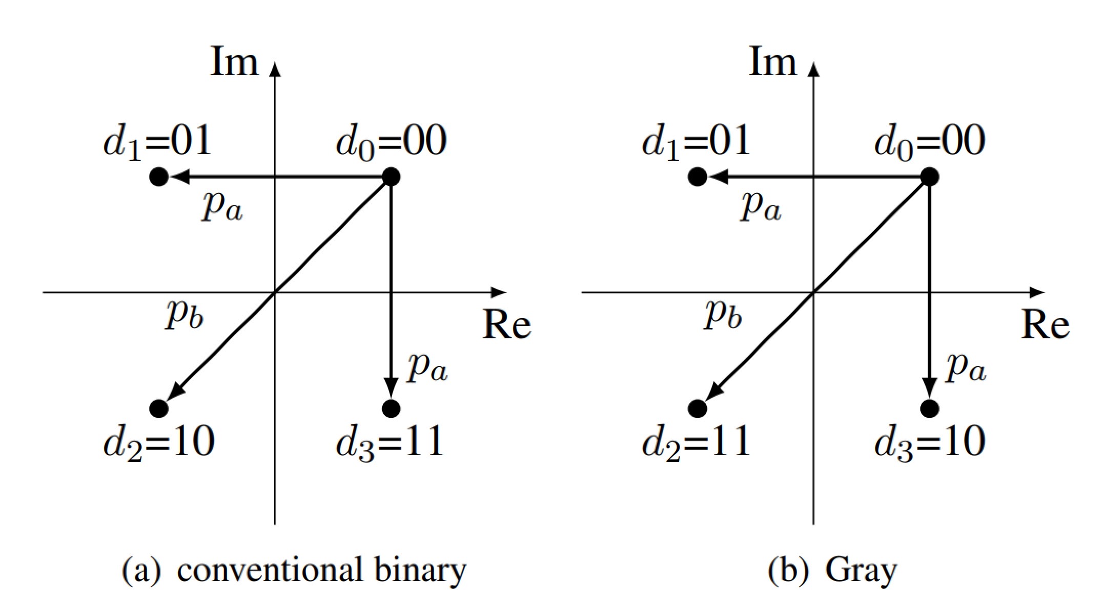
What difference in BER do we have between Gray code and conventional binary code?

For larger  , Q(⋅) becomes small and can be neglected, leading to

A signal space is a vector space with finite dimension. The vectors  are orthagonal when the inner products between two different vectors is zero and with the same vector one.
  stands for the inner product of psii(t) and ψj(t).

A signal vector is:

with
![[ ]
ai1 ai2⋅⋅⋅aiN](main2_for_html110x.svg)

 2 = ∑
j=1Na
ij2
2 = ∑
j=1Na
ij2To determine how efficient our protocol is one can calculate the average energy per symbol as below.

z(t) was at any point in time whereas z(T) is at a specific sample point, when we sample once per symbol time T is the symbol time. The last box in the plot above is the test statistic, dependent of the value of z it will say the signal is one or zero.
When one sends symbol zero one receives the following without noise a0(T) = s0(t) * h(t)|t=T and when sending symbol one the following a1(T) = s1(t) * h(t)|t=T . For the noise part one gets the following n(T) = (n)(t) * h(t)|t=T , since our filter is linear, we get again a Gaussian process, so nothing changes. The Gaussian signal can be described with the following formula:

For the test statistic we get the following: z(T) = ai(T) + n(T) and since a Gaussian signal + a constant gives another gausian signal, but with another mean we can describe it like the following: z(T) = N(ai(T), σ2)
So the probability density function of z(T) if ”0” was sent is the following:


As one can see below, there are different types of modulations
alphabet or constellation ⇒ is a collection of symbols, the alphabet for a bit would be zero and one.
In a digital communication system, we want to transmit something digitally, but normally the original signal is analog like voice, therefore one has to digitize it and afterwards to transmit it we normally put it into analog again, because normally one can not transmit the signal digitally.
One transmits the original signal with multiple bits.
I want to transmit the data from a 3bit ADC ⇒ we have eight different codes. With this modulation we transmit three different bits.
One transmits the original signal with different amplitudes. Here we have a symbol rather than a binary bit.
I want to transmit the data from a 3bit ADC ⇒ we have eight different codes. To transmit this signal I generate 8 different amplitudes.
To transmit the same amount of data PCM must have much higher frequencies than PAM (in the example above it must be three times larger, because in the same amount of time we must transmit three bits) ⇒ PCM uses a larger bandwidth. But there are a lot more line codes as can be seen blow and each one of those is good at a very specific thing. (Clock recovery, error detection, differential coding, etc.)
Spectral efficiency ⇒ η =  ← system bit rate ∕ system BW
 , Tb : bit duration
 Tb
Tb

When we simplify the schematic above, we get a sampling receiver
A Wiener filter minimizes the mean-square error to a minimum.
The output of the filter in the diagram above can be described as the following:
![M
∑
sˆ[n + D ] = wi ⋅ y [n - i]
i=0](main2_for_html124x.svg)
![[w1, w2,...,wN ]](main2_for_html125x.svg) T
T
![[s1,s2,...,sk]](main2_for_html126x.svg) T
T
Let’s assume one has a filter with three filter coefficients w0, w1, w2. The output can then be written in the following form:
![ˆs[0] = w0y [0]
ˆs[1] = w0y [1] + w1y[0]
ˆs[2] = w0y [2] + w1y[1] + w2y[0]
ˆs[3] = w0y [3] + w1y[2] + w2y[1]](main2_for_html127x.svg)
Where ˆs [k] can also be written as A[k]w where A[k] is the following:
![( )
| y[0] 0 0 |
| y[1] y[0 ] 0 |
A [k] = || y[2] y[1 ] y[0] ||
|( .. .. .. |)
. . .
y[k] y[k - 1 ] y[k - 2]](main2_for_html128x.svg)
and w ≜![[w1, w2,...,wN ]](main2_for_html129x.svg) T the error can then be written as:
T the error can then be written as:
![e[k] = s [k ] - y[k] = s[k] - A [k]w [k ]](main2_for_html130x.svg)
The error is minimized when the following condition is given:
![( T )- 1 T
w [k ] = A [k]A [k] A [k]s[k]](main2_for_html131x.svg)
When rewriting this we end up with the following equation:

which is also called the wiener-hopf equation. Also note that R is the autocorrelation with the input signal
![( )
γyy[0] γyy[- 1] ⋅⋅⋅ γyy[- M ]
| γ [1] γ [0] ⋅⋅⋅ γ [1 - M ] |
Ryy = || yy. yy. yy . ||
( .. .. .. )
γyy[M ] γyy[M - 1] ⋅⋅⋅ γyy[0]](main2_for_html133x.svg)
and p or also rsy the cross-correlation of the input and the chennel output.
![( )
| γsy[D ] |
| γsy[D + 1] |
rsy = |( ... |)
γsy[D + M ]](main2_for_html134x.svg)
What is h[n] of the first part in Figure 25?
Figure 25 shows that the first part is an IIR Filter with h[n] = αn ⋅ ϵ[n]
Lets assume α is -0.5. How does H[z] and it’s inverse look like?
We know the following:
h (n) (n) | = αn ⋅ ϵ[n] ϵ[n] | ||
| X(z) | =  |

Therefore X(z) =  and X(z)-1 = 1 - α ⋅ z-1
X (z)-1 (z)-1 | = 1 - α ⋅ z-1 z-1 | ||
| h-1[n] | = 1 ⋅ δ[n] - α ⋅ δ[n - 1] |

With this information we know that the inverse of h[n] is an FIR filter with the impule response of 1 ⋅ δ[n] + 0.5 ⋅ δ[n - 1]. w0 should therefore be one and w1 0.5 when one assumes that s[n] is white noise and n[n] is zero.
What do we get when we use the wiener filter?
![1 1 1 1 k 1 4 2
γss[0] = 1 +--+ ---+ ---... = (-) = -----1- = --= 1.33 = σx
4 16 64 4 1 - (4) 3
1- 2-
γss[1] = γss[0] ⋅ (- 2) = - 3 = - 0.666
1 1
γss[2] = γss[1] ⋅ (--) =-= 0.333
2 3](main2_for_html144x.svg)
![(
|{ σ2s + σ2n if m = 0
γ [m] = γ [m ] + γ [m ] = - 2 if |m | = 1
yy ss nn |( 3
13 if |m | = 2](main2_for_html145x.svg)

Since we know the following: x[n] = a ⋅ x[n - 1] + s[n] ⇒ s[n] = x[n] - a ⋅ x[n - 1] we can calculate rsy with
![⌊⌈ E (s[n ] ⋅ y[n]) ⌋⌉
rsy = E (s[n ] ⋅ y[n - 1])
E (s[n ] ⋅ y[n - 2])
⌊ E ((x [n ] - a ⋅ x[n - 1]) ⋅ y[n]) ⌋
⌈ ⌉
= E ((x[n ] - a ⋅ x[n - 1]) ⋅ y[n - 1])
E ((x[n ] - a ⋅ x[n - 1]) ⋅ y[n - 2])
⌊ E ((x [n ] - a ⋅ x[n - 1]) ⋅ (x[n] + v[n ])) ⌋
⌈ ⌉
= E ((x[n ] - a ⋅ x[n - 1]) ⋅ (x[n - 1] + v[n - 1]))
E ((x[n ] - a ⋅ x[n - 1]) ⋅ (x[n - 2] + v[n - 2]))
⌊ E (x[n ] ⋅ x[n] + x[n] ⋅ v[n] + x[n] ⋅ (- a) ⋅ x[n - 1] + v[n] ⋅ (- a ⋅ x�
⌈ ⌉
= E (x[n] ⋅ x[n - 1] + x[n] ⋅ v[n] + x[n - 1] ⋅ (- a) ⋅ x [n - 1 ] + v[n] ⋅ (- a &
E (x[n] ⋅ x[n - 2] + x[n] ⋅ v[n] + x[n - 2] ⋅ (- a) ⋅ x [n - 1 ] + v[n] ⋅ (- a &
42 42
| E 3 +(0 + - a ⋅ a ⋅ 3)+ 0 |
= || E a ⋅ 42 - a ⋅ 42 ||
⌈ ( 3 3 ) ⌉
E a2 ⋅ 42 - a2 ⋅ 42
⌊ ⌋ 3 3
1
= ⌈ 0⌉
0](main2_for_html147x.svg)

Lets assume we have again a system as one can see in Figure 25 where s[k] and n[k] are white gaussian with zero mean. Furthermore they are uncorrelated E{s[k]n[k] = 0}. Lets also assume that:
![{ } { }
E x2 [k] = σ2x and E n2[k] = σ2n](main2_for_html149x.svg)
What is
![{ 2 }
E y [k ] ,E {y[k]y [k - 1]},E {x[k]y[k]},E{x [k]y [k - 1]}](main2_for_html150x.svg)
Since E![2
{x [k]}](main2_for_html151x.svg) and E
and E![2
{n [k]}](main2_for_html152x.svg) are given
are given
![{ } { } { }
E y2[k] = E x2[k ] + 2 E {x[k]n [k ]} +E n2[k] = σ2x-+-σ2n-
◟----◝=◜0---◞](main2_for_html153x.svg)
and
![E {y [k]y[k - 1]} = E {x[k]x [k - 1]} + E {x[k]n[k - 1]} + E {x[k - 1]n[k]} + E {
◟------◝◜------◞ ◟------◝◜------◞ ◟------◝◜------◞
=0 =0 =0
= E {x[k]x [k - 1]} = aσ2x
----](main2_for_html154x.svg)
and
![{ }
E {x[k]y [k]} = E x2[k] + E {x [k ]n [k]} = σ2x-
◟ ---◝◜----◞
=0](main2_for_html155x.svg)
and
![2
E {x[k]y[k - 1]} = E{x [k ]x [k - 1]} + E◟-{x[k]n◝[◜k --1]}◞ = a-σx
0](main2_for_html156x.svg)
Therefore
![( E {y2[k]} E {y[k]y2[k - 1]} ) ( w0 ) = ( E{x [k ]y[k]} )
E{y [k ]y[k - 1](} E {y [k]} ) ( w1 ) ( E{x [k) ]y[k - 1]}
σ2x + σ2n aσ2x w0 σ2x
a σ2 σ2 + σ2 w = aσ2
( x 2 x n ) ( 1 ) ( x)
1 + σn2 a w0 1
σx σ2n w = a
a 1 + σ2 ( 1 ) ( )
w0 1
=
w1 a ( )
( w ) 1 1 + σ2n2 - a ( 1 )
0 = (-------)2----- σx σ2n
w1 1 + σ2n2 - a2 - a 1 + -σx2 a
σx ( )
1 + σ2n - a2
= (------1)------( σ2x( 2) )
1 + σ2n 2 - a2 - a + a 1 + σσn2
σ2x x](main2_for_html157x.svg)
Adaptive filters are divided in the following applications:
LMS-Based adaptive filters are based on wiener filters (linear prediction). But instead of calculating the coefficients w directly, it calculates them interactively.
| (19) |
lms_filter(0.1,2,[1,1,1,1,1,1,1],[1,1,1,1,1,1,1])

function [e,w]=lms_filter(mu,M,x,d)

    % [e,w]=lms_filter(mu,M,x,d)

    % Inputs:

5    % mu = step size, dim 1x1

    % M = number of filter coefficients, dim 1x1

    % x = input signal, dim Nx1

    % d = desired signal, dim Nx1

    %

10    % Outputs:

    % e = estimation error, dim Nx1

    % w = final filter coefficients, dim Mx1

    e = zeros(size(x)); %preallocate

    w = zeros(M,1); %preallocate

15    x = x(:); d = d(:); %ensure column vectors

    for k=M:length(x)

        xvec = x(k:-1:k-M+1);

        e(k) = d(k)-w’*xvec; %compute error

        w = w + mu*e(k)*xvec; %LMS update

20    end

end
![[ ]
1
1](main2_for_html159x.svg) , e =
, e = ![[0 1 0 0 0 0 0 ]](main2_for_html160x.svg) and w =
and w = ![[ ]
0.1
0.1](main2_for_html161x.svg)
![[ ]
1
1](main2_for_html162x.svg) , e =
, e = ![[ ]
0 1 0.8 0 0 0 0](main2_for_html163x.svg) and w =
and w = ![[ ]
0.18
0.18](main2_for_html164x.svg)
![[1]
1](main2_for_html165x.svg) , e =
, e = ![[ ]
0 1 0.8 0.64 0 0 0](main2_for_html166x.svg) and w =
and w = ![[0.244]
0.244](main2_for_html167x.svg)
Converges faster than lms algorithm.
| (20) |
For statistics and control theory, Kalman filtering, also known as linear quadratic estimation (LQE), is an algorithm that uses a series of measurements observed over time, including statistical noise and other inaccuracies, and produces estimates of unknown variables that tend to be more accurate than those based on a single measurement alone, by estimating a joint probability distribution over the variables for each timeframe. The filter is named after Rudolf E. Kálmán, who was one of the primary developers of its theory.
To understand a callman filter one must be familiar with the mean, covariance and correlation of a time series.

To calculate the next sample in a kalman filter one must know what the following variables mean:
Furthermore one must be familiar with the state space reperesentation. Thereby the following video series is very helpful. For a Kalman-Filter one can use the following recipe:
 -1
-1

 Pk∣k-1
| (21) |
| (22) |
| (23) |
| (24) |
| (25) |
| (26) |
You are given a linear, shift-invariant system as depicted above. This system has the scalar state xk and produces the scalar output yk at every discrete time instant k. The measurement-noise vk and the process-noise uk are zero-mean Gaussian random variables with Rk = E{vk2} = 1 and Q k = E{uk2} = 1.


First one has to calculate kk which can be done with Equation 22. From Figure 27 we know that C = 1, Pk∣k-1 =  and Rk = 1. Therefore

In the next step one can calculate xk∣k with the new measurement yk, therefore and due to Equation 23

With Equation 21 one can now calculate Pk∣k.

In the next step, one can calculate Pk+1∣k with Equation 24

With Equation 26 one can calculate xk+1

Now one can repeat the steps before and one gets the following result:

Now one can repeat the steps before and one gets the following result:


Alternatively, one can also program a program on the ti-nspire and call it then like the following:
sign_proc\kalman(1,1,((4)/(3)),0,[((1)/(2))],[1],[1],((4)/(5)))
sign_proc\kalman(Rk,Qk,Pk|k-1,xk|k-1,A,B,C,yk)
which outputs then the following:
Rk : 1, Qk : 1, Pk|k-1 : ((4)∕(3)), xk|k-1 : 0, A : [((1)∕(2))], B : [1], C : [1], yk : ((4)∕(5)) kk = [((4)∕(7))], xkk = [((16)∕(35))], pk|k = [((4)∕(7))], xk+1|k = [((8)∕(35))], pk+1|k = [((8)∕(7))]
The program itself looks like the following:
Define LibPub kalman(r_k,q_k,pkk_m_1,xkk_m_1,a,b,c,y_k)=
Prgm
:©Inputs a(R_k (covariance of observation noise), R_k (covariance of the proccess noise), pkk_m_1,xkk_m_1, a,b,c,y_k)
:Disp "R_k: ",r_k,", Q_k: ",q_k,", P_{k|k-1}: ",pkk_m_1,", x_{k|k-1}: ",xkk_m_1," , A: ",a," , B: ",b," , C: ",c," , y_k: ",y_k
:Disp " "
:Local k_k,x_k_k,p_k_k,xkk_p_1,pkk_p_1
:k_k:=pkk_m_1*c^T*(c*pkk_m_1*c^T+r_k)^(-1)
:x_k_k:=xkk_m_1+k_k*(y_k-c*xkk_m_1)
:p_k_k:=(identity(max(dim(c)))-k_k*c)*pkk_m_1
:xkk_p_1:=a*x_k_k
:pkk_p_1:=a*p_k_k*a^T+q_k
:Disp "k_k=",k_k," , \hat{x}_{k_k}=",x_k_k," , p_{k|k}=",p_k_k," , x_{k+1|k}=",xkk_p_1," , p_{k+1|k}=",pkk_p_1
:PassErr
:EndPrgm
Lets assume we want to measure the position of an airplane, with v0x = 280 and x0 = 4000 m.


Process Errors i Process covariance matrix


Our estimate of Xkp which is the next state is the following:
![Xkp = AXk -1 + Buk + wk
[ 1 Δt ] [ x0 ] [ 1Δt2 ]
= + 2 [ax0] + 0
[ 0 1 ][ v0 ] [ Δt ]
1 1 4000 1∕2 [ ]
= 0 1 280 + 1 2
[ ] [ ]
= 4280 + 1
280 2
[ ]
Xkp = 4281
282](main2_for_html197x.svg)
Initial Process Covariance The cross term is often set to zero, since they are independent of each other.
![[ 2 ] [ ]
P = Δx Δx Δv = 400 100
k-1 Δx Δv Δv2x 100 25
[ ]
Pk-1 = 400 0
0 25](main2_for_html198x.svg)
The predicted process covariance matrix
![⊤
Pkp = APk - 1A + QR
[ 1 Δt ] [ 400 0 ] [ 1 0 ]
= + 0
[ 0 1 ][ 0 25] [ Δt ]1
1 1 400 0 1 0
= 0 1 0 25 1 1
[ ] [ ]
400 25 1 0
= 0 25 1 1
[ ] [ ]
= 425 25 ⇒ 425 0
25 25 0 25](main2_for_html199x.svg)
![---PkpH--⊤----
K = HPk H ⊤ + R
p [ ] [ ]
425 0 1 0
---------------0---25-----0--1---------------
= [ 1 0 ] [ 425 0 ] [ 1 0 ] [ 625 0 ]
+
0 1 [ 0 25] 0 1 [ 0 36]
425 0 425 0
0 25 0 25 [ ]
= [----------]---[---------]-= [-----------] = 0.405 0
425 0 625 0 1050 0 0 0.410
0 25 + 0 36 0 61](main2_for_html200x.svg)
![Yk = Cyk + Zk
[ 1 0 ][ 4260 ]
Yk = + 0
[ 0 1 ] 282
4260
Yk = 282](main2_for_html201x.svg)
![X = X + K [Y - HX ]
k [ kp ] [ k kp ] ( [ ] [ ] [ ])
4281 0.405 0 4260 1 0 4281
= 282 + 0 0.410 282 - 0 1 282
[ ] [ ] [ ]
= 4281 + 0.405 0 - 21
282 0 0.410 0
[ 4281 ] [ - 8.5 ]
= +
2[82 ] 0
4272.5
Xk = 282](main2_for_html202x.svg)
![Pk = ([I[ - KH )]Pkp[ ][ ][ ]
1 0 0.405 0 1 0 425 0
Pk = 0 1 - 0 0.410 0 1 0 25
[[ ] [ ][ ]
P = 1 0 - 0.405 0 425 0
k 0 1 0 0.410 0 25
[ ] [ ]
k = 0.595 0 425 0
[ 0 0.590] 0 25
253 0
Pk = 0 14.8](main2_for_html203x.svg)
![[ 4272.5 ]
Xk = ⇒ Xk -1 ⇒ Xkp = AXk -1 + Bk + wk
[ 282 ]
253 0 ⊤
Pk = 0 14.8 ⇒ Pk- 1 ⇒ Pkp = APk -1A + Qk](main2_for_html204x.svg)
The idea behind this system is that all transmitters use the same time and frequency allocation. To distinguish the different users, a code is assigned to each of them. The code is then used to spread a small information bandwidth over the much wider channel bandwidth. CDMA is thus a spread spectrum (FH-SS) technique. There are two ways to do that, one is frequency hopping (FH-SS) and the other is by multiplying the data sequence with a much higher chip sequence (DSSS), as one can see in Figure 29.
The spreading gain of such a system can be calculated according to Equation 27, where the bit time is called Td and the chip time Tc.
| (27) |
CDMA (Code Division Multiple Access) is a wireless communication technology that uses unique codes to separate different signals in the same frequency band. It was mainly used in some areas for 2G and 3G cellular network technology.
Spreading is the process of assigning a unique code to each user’s data to distinguish it from other users’ data. The receiver then applies the same code to decode the intended data (For that one uses the m-sequences (Glonass), Gold codes (e.g. GPS)). Spreading allows multiple users to share the same frequency band simultaneously by separating their signals through code division. This results in an increase in the number of users that can access the network and improves the overall network capacity. (When doing this, one increases the bandwidth (frequency))
Is the most prominent communication system in Europe. As opposed to GSM and other TDMA-based cellular systems, where one user has a link to one cell only at one given time, a UTMS user can use signals from two base stations. They send with the same user code, such that the signal looks as if it was sent through a multipath environment. Thus, we do not have a hard handover when changing from one cell to another, but rather a smooth, so-called soft handover, where the user may have a simultaneous link to two base stations during a transition phase
Hadamard matrix / Walsh matrices are used to generate the code for the different users in a system as it can also be seen in subsubsection 12.2.5. The equation to calculate the Hadamard matrix can be found in Equation 28. To do the calculation one must know the Kronecker Product (⊗) to which an example can be found in Equation 29. An important property of the Hadamard matrix is that when one multiplies two rows with each other and ads them up the result is always zero see also Equation 30. In the end one multiplies the signal for a certain user with one column of the matrix. The receiver (user) does the same and is then able to decode the signal.
| (28) |
| (29) |
The carrier-to-interference ratio (C/I) in CDMA refers to the ratio of the power of the desired signal to the power of the unwanted interference in the system. A higher C/I ratio indicates a better signal quality and a lower level of interference, which can result in improved system performance and capacity. For example a carrier-to-interference ratio (C/I) of 1000 means that the power of the desired signal is 1000 times greater than the power of the unwanted interference. This indicates that the signal quality is very good and there is a low level of interference in the system. A high C/I ratio is desirable in CDMA communication systems as it results in improved system performance and capacity. A C/I ratio of 1000 is considered very high and provides excellent signal quality and minimal interference.
Construct the Hadamard matrix H8 and check the orthogonality property of the codes given by row 2 and row 8, respectively.

| (30) |
Now let us assume a CDMA system with a data rate of 125 kbit/s (BPSK with a �1 data stream), a chip rate of 1 Mchip/s and a carrier frequency of fc. Sketch the transmitter of such a system and assign important parameters.
Sketch the receiver of such a system and assign important parameters.
See Figure 29
Sketch the receiver of such a system and assign important parameters.
See Figure 29
Draw in a qualitative way the amplitude spectrum around the RF carrier of the RF signal with only data modulated (no spreading).
Since the pulse duration is 8 × 10⁻⁶ s and the Fourier transform of a rectangle is |T|⋅ si(πTf) = 8 × 10⁻⁶ one can draw the graph. Important to know is that when one solves the following equations
 = 0 ⇒ 8 × 10⁻⁶ s ⋅ π ⋅ f = π one gets 125 × 103 Hz which is half of the null to null bandwidth ⇒ the null to null bandwidth is 250 × 103 Hz, see Figure 30.
Draw in a qualitative way the amplitude spectrum around the RF carrier of the spread RF signal
Since the pulse duration is 1 × 10⁻⁶ s and the Fourier transform of a rectangle is |T|⋅ si(πTf) = 1 × 10⁻⁶ one can draw the graph. Important to know is that when one solves the following equations
 = 0 ⇒ 1 × 10⁻⁶ s ⋅ π ⋅ f = π one gets 1 × 10⁶ Hz which is half of the null to null bandwidth ⇒ the null to null bandwidth is 2 × 10⁶ Hz,see Figure 31.
What is the spreading gain
According to Equation 27 it is GdB = 10 log 10 = 10 log 10
 ≈ 9dB. The spreading factor would be 8 since the frequency was increased by 8. But this also means the power density maximum has decreased by a factor of 9dB.
Walsh code should be used with a spreading factor of four and two users should use the channel at the same time. We know from Equation 28 that with a spreading factor of four we get the following matrix1:

One now has to assign to each user one code. Let’s say 20!//user one has row one and 20!//user two row two. The other rows are inactive.
Let’s assume the Data of the users are the following:

This gives then the following 20!//code sequence:
1 | 1 | 1 | 1 | ∣1 | 1 | 1 | 1 | ∣- 1 | -1 | -1 | -1 | ∣- 1 | -1 | -1 | -1 | ∣1 | 1 | 1 | 1 | ∣- 1 | -1 | -1 | -1 | |
-1 | 1 | -1 | 1 | ∣- 1 | 1 | -1 | 1 | ∣1 | -1 | 1 | -1 | ∣- 1 | 1 | -1 | 1 | ∣- 1 | 1 | -1 | 1 | ∣1 | -1 | 1 | -1 | |
0 | 2 | 0 | 2 | ∣0 | 2 | 0 | 2 | ∣0 | -2 | 0 | -2 | ∣- 2 | 0 | -2 | 0 | ∣0 | 2 | 0 | 2 | ∣0 | -2 | 0 | -2 |
The receiver does then a sequence
wise multiplication with the received data and the assigned walsh-code, which is for user one 1111.
0 | 2 | 0 | 2 | ∣0 | 2 | 0 | 2 | ∣0 | -2 | 0 | -2 | ∣- 2 | 0 | -2 | 0 | ∣0 | 2 | 0 | 2 | ∣0 | -2 | 0 | -2 | |
4 | ∣ | 4 | ∣ | -4 | ∣ | -4 | ∣ | 4 | ∣ | -4 | ||||||||||||||
As one can see from the result above one gets the exact same data as one has transmitted.
We do frequency hopping so that if we have interference on a certain frequency, for example from a microwave, one can still receive and send data some data and not all is lost, but only some. To do this the transmitter and receiver are hopping in the same rhythm from one frequency to the other. Fast FHSS (Frequency hopping spread spectrum) means that one bit gets transmitted over multiple frequencies is not used, because one would need to switch the frequency very fast. Slow FHSS each bit gets transmitted over one frequency ⇒ Hamming can be used to reconstruct false ones.
What is spreading gain?
See Equation 27
What is cell breathing?
In CDMA-based Cellular networks, cell breathing is a mechanism which allows overloaded cells to offload subscriber traffic to neighbouring cells by changing the geographic size of their service area. Heavily loaded cells decrease in size while neighbouring cells increase their service area to compensate. Thus, some traffic is handed off from the overloaded cell to neighbouring cells, resulting in load
balancing.
The signal-to-noise ratio given by thermal noise is usually designated as SNR. The corresponding signal-tonoise ratio due to interference by other users on the same channel is described by C/I (carrier-to-interference ratio).
Now consider the following situation. A certain CDMA system can live with an SNR of 10 dB, if no additional interference is present.
 = 2).
= 2).
If spreading codes can be chosen such that a concurrent transmitter produces a C/I of 1000/1, how many transmitters can transmit simultaneously if the total signal-to-noise-plus-interference-ratio SINR is not to fall below the original 10 dB? The SINR is given by the linear measure

SINR stands for Signal-to-Interference-plus-Noise Ratio in CDMA. It is a measure of the quality of a received signal compared to the combined power of all other interference signals and background noise. A high SINR indicates a strong signal and low interference and noise, while a low SINR indicates weak signal quality and high levels of interference and noise. SINR is an important performance metric in CDMA communication systems as it directly impacts the ability to accurately recover the intended signal. A high SINR results in improved system performance and capacity, while a low SINR can lead to errors and degradation of system performance.
Can you allow more simultaneous transmitters for the same SINR by increasing all transmitter powers?

Where are the limits?
Maximum-length sequences have very interesting autocorrelation properties: they have one peak for exact alignment, and the same low level for misalignment of one or more chips.
| (31) |
A signal is consider as ultra wide band when ν from Equation 32 is larger than 20%
| (32) |
OFDM has the benefit that frequency-selective fading is no problem and no spectrum is wasted for guard bands. Nevertheless, guard intervals are inserted to prevent ICI(inter channel interference) The following video might be helpful. The equalizer is in the frequency domain, and therefore it is much easier.
The total excess delay is the total difference from the first and last signal received through the channel due to reflection. The mean delay of a received signal can be calculated according to Equation 33, where PT is the power of the transmitted signal and can be calculated according to Equation 35. The delay spread can be calculated according to Equation 34 and is dependent on Equation 35 and Equation 33. The delay spread has quite an important
role in OFDM, since it defines the guard intervals.
| (33) |
| (34) |
| (35) |
What is the mean delay of a channel with the impulse response of h(t) = δ(t) + 0.5δ and T1 = 1μs?

What is the spread of the signal mentioned above?

How would the frequency response look like obtained in the Fourier domain?

Draw the spectrum:


Compute the coherence bandwidth of this channel and compare it with your estimated value:
Depending on the definition we either have

or, if the correlation function (among the impulse response at the different frequency positions) is to be > 0.9

Given is a wirless system with the following parameters:
 =
=  ⇒ v =
⇒ v =  ⋅
⋅ =
=  ⋅
⋅ = 3.36 × 10³ m s-1, since T
coh ≫
= 3.36 × 10³ m s-1, since T
coh ≫ =
=  = 3.2 �s. Therefore it is long enough (speeds in a room that are larger than 3.36 × 10³ m s-1 is not common)
 . Furthermore τRMS =
  (the delay spread is the length spread of the different paths divided by the speed of light). With Equation 40 one can write Bcoh ≈
 ≫
≫ =
=  = 312.5 kHz ⇒
 ≫= 312.5 kHz ⇒
 ≫ xRMS ⇒ 19.2 m ≫ xRMS which is plausible for a normal room.
| (36) |
| (37) |
fd=Doppler spread (when we head to the transmission station with our phone, we get a doppler effect, fRF (center frequency) gets higher, doppler spread is normally in the range of Hz (a few hertz)), see also Equation 38
| (38) |

The formula below is in our signal
| (39) |
It’s important to have the following in mind: When one has a small bandwidth the signal gets long (for a sharp impulse one needs a huge bandwidth (UWB)). One now has to find a number of sub carriers Nc that make the bandwidth not to small (Nc not to large) ⇒, otherwise the time gets to long (problems with moving objects) and do not make them to wide (Nc not to small)⇒, otherwise frequency fading could cause issues. The behaviour can be described with Equation 40.
| (40) |
Furthermore one must be aware of the following Rule of Thumbs: Equation 41 can be used if the frequency correlation function is above 0.9.
| (41) |
Equation 42 can be used if the frequency correlation function is above 0.5.
| (42) |
Equation 43 is sometimes also used (leading to yet another value for the correlation function).
| (43) |
Very similar rules can be found for the relationship given by Equation 36(for the time correlation to be above 0.5), see also Equation 38 for the Doppler spread .
| (44) |
With those equations one could make the following statement for coherence times of about 0.5.

Exercise: For 802.11a (WLAN), we have W = 20MHz and Nc = 64. What is the subcarrier distance? How large should Bcoh and Tcoh of the channel be at least?
The subcarrier distance is:


FFT is a circular and not a linear convolution.

In OFDM we have a lot of sub carriers, and all sub carriers are orthogonal.
Shannon’s channel capacity:
| (45) |
In a multicarrier system:

Power Received:
| (46) |
| (47) |
| (48) |
Example: Imagine a two-carrier system with total power P = P1 + P2. If the two channel coefficients H1 and H2 are given, derive the choice of P1 and P2 that optimize the use of the channels. With Equation 45 and Equation 46 one can create the following equation system:

Since we want to have it’s maximum, one has to derive it and then set it to zero.
With some magic we end then with the following:

When P1 is negative, we do not assign any energy to it.
The DAB system (digital audio broadcast) facilitates different OFDM Transmission modes to allow for some flexibility with respect to environment and change of environment (due to vehicle movement). Assume a total bandwidth of W = 1.536 MHz. Complete the following table:

What efficiency (with respect to the guard time ’wasted’) does the OFDM system have?

State the numerical condition for the coherence bandwidth for TM I According to Equation 40:

With the rule of thumb that the delay spread and the coherence bandwidth are related through state the condition for the delay spread for TM I.

one gets:

State the numerical condition for the coherence time for TM I. According to Equation 40:

With the rule of thumb that (for a correlation coefficient of 0.5) the coherence time is in relation with the Doppler frequency shift is as in the euqation below. Compute the coherence time for a vehicle speed of 120 km/h and an RF of 1.5 GHz (L-band as used in DAB).

The Doppler frequency can be calculated according to Equation 49
| (49) |

Is the coherence-time condition satisfied sufficiently for TM I? . TM I is suitable for large delays but slow vehicle speed. TM III is better suited to high-speed, but allows only moderate delay spreads.
As one can see in Figure 35 the average energy (Pavg) of the sub carriers is Nc ⋅ Psub. But the peak energy PPeak is (Nc ⋅ xn)2, which is much higer. Therefore it is possible that one has some very high peaks in an OFDM system.
Imagine an OFDM system with 8 subcarriers of BPSK modulated signals, each with power Psub. The absolute highest peak possible for such a signal can therefore be 8 times the value of one isolated subcarrier.
Compute the average power, the peak power and thus the peak-to-average-power value.

If we have one redundant channel, i.e., we can choose the eighth channel to reduce the amplitude of the composite signal, what reduction in the peak-to-average-power value would we get?
The idea is to sent a minus one when all other channels send a one and vice versa, therefore the max amplitude reduces to 6 ⋅ xmax

Very often, not the highest peak is considered, but the percentage that a certain amplitude is exceeded. Compute for the original 8-subcarrier OFDM system, the probability that the signal exceeds 3 times the amplitude of a single subcarrier.
On the TI-Nspire you find the binomial coefficient under menu→5:Probability →3: Combinations ⇒ nCr
Furthermore one knows from Equation 89 that the following holds:

Therefore

since the amplitude is larger than 3 when 6,7 or 8 subcarriers show a one (when only 5 subcarriers show a one one has 5-3=2, which is less than one).

Compute for the OFDM system with one subcarrier chosen such as to lower the amplitude, the probability that the signal exceeds 3 times the amplitude of a single subcarrier.

Since mostly error occur in bursts, it turned out that interleaving is good.

When one does interleaving and apply an error correction code again on the deinterleaved signal one can detect/correct much more errors since they are distributed to different regions.
The goal of trellis modulation is to consider modulation and error correction in the same approach. Most trellis modulation approaches have one additional bit. Note, one does not increase the bandwidth or the bitrate. The mind distance and the min free path can be calculated with the folwoing formulas:
| (50) |
| (51) |
A good video can be found under the following link
Given is the following convolutional code for the last two bits, it can also be seen in Figure 35a:
With this information one is then able to draw the set-partitioning as it can be seen in Figure 35e. There one looks that the most significant bit is always the furthest apart. The most significant bit is not coded.
With this information, one can then draw the trellis, see also Figure 35b. When the state is [0,0] (storage element is [0,0]) and we insert the vector x = {x, 0} we stay in the same state, since the value from the storage does not change. Otherwise, when we insert the vector x = {x, 1} We change the state since the storage element is then [1,0]. With this, one can then draw the whole
graph.
To calculate the coding gain according to Equation 53 one has to calculate first the value of dmin,uncoded 2. For that, one can use the formula from paragraph 16.1.2, which says: d
min2 =  . Duet to that dmin,uncoded 2 =
  and dmin,coded 2 =
  . This means that A is
  ∕2 =
∕2 =  . The dfree,coded 2 can be searched with the trellis in Figure 35c. The distance is then
  ⋅
⋅ 2 =
2 =  . The gain is then
10 log 10(
. The gain is then
10 log 10( ) = 3.3dB, due to the fact that the gain can be described with the following formula:

1/2 mans one has one input and two outputs.
| (52) |
The number of states of a trellis is always given by two to the power of number of storage elements, for example Figure 40 has two states, since 21 = 2. The coding gain G is given by Equation 53.
| (53) |
When one wants to calculate the coding gain for a two-state 2/3 TCM with QPSK one gets the following result:

This is because the shortest distance squared in QPSK is 2, see also Figure 37, when one sends one bit the shortest distance squared is two, since one would go from position zero to position two in Figure 37. In a two-state 2/3 TCM it looks different, one has a storage element, due to that the signal looks like in Figure 38 when one changes the LSB. This results in a total distance of dfree 2 = d2(0, 2) + d2(0, 1) = 2 + (2 - ) = 2.5858 (Note to
calculate the distance one always refers to zero as it is also done in subsubsection 15.0.1). When one would change the most significant bit the distance would be even higher, since one jumps always to the other side of the circle.
) = 2.5858 (Note to
calculate the distance one always refers to zero as it is also done in subsubsection 15.0.1). When one would change the most significant bit the distance would be even higher, since one jumps always to the other side of the circle.
LectureNotes 2022 part1-135.png 
LectureNotes 2022 part1-137.png 
LectureNotes 2022 part1-137.png
See also the following video. We have an input signal x1 = {0, 1, 0} and x2 = {0, 1, 0} and the received values are n1 = 0, n2 = -0.8 + j, n3 = 0. We start at state zero and calculate now the distances to the other states. Since we received zero in the beginning, the squared distance to zero is zero, to four four, to two two and to six also two. In the next state we received -0.8 + j, therefore, the distance to zero is
(1 --0.8)2 + (0 - 1)2 = 4.24, to point four (-1 --0.8)2 + (0 - 1)2 = 1.04, to point one ( --0.8)2 + (
 - 1)2 = 5.07 and so on. for the last received signal one can do again the same. In the end one decides for the path which has the least squared distance, which is 0,6,1. This is also what was sent according to subsubsection 15.0.4. The whole diagram can be found in Figure 42
| Bit | State1 | State2 | State3 |
| MSB | 0 | 1 | 0 |
| 0 | 1 | 0 | |
| LSB | 0 | 0 | 1 |
| Result | 0 | 6 | 1 |
entropy:
| (54) |
conditional entrpy:
| (55) |
The capacity is then given as:
| (56) |
When one has a gaussian distributed signal and gausian distributet noise the max capacity is given with the formula below.
| (57) |
For a discrete memoryless channel (DMC) the following applies.
| (58) |
where p(x) is the distribution for example zero and one with a dirac of 1/2 at each point. Numerical evalution for the capacity.
| (59) |
The average symbol and Bit energy in QAM and PSK is given by Equation 60.
| (60) |
Where:
Given is the M=8 rectangular QAM that can be seen in Figure 44
now one wants to calculate Es, Eb. This can be done with Equation 60 this gives the following result (see also the following video).
![M -1
-1- ∑ 2 -Joules--
Es = M |sm | Symbol
m=0
1-[( 2 2) ( 2 2) ]
= 8 A + A 4 + (3A ) + A 4
1 [ ]
= -- 8A2 + 40A2
8
= 48-A2 = 6A2
8
-6A2-- 2
Eb = log 8 = 2A
2](main2_for_html326x.svg)
Where:
Example derive the minimum Euclidean distance dmin2 in an M-array PAM system, whose power has been normalized to one
With Equation 60 one can calculate the energy per symbol (as a reference also have a look at Figure 45):

Since we want P = 1, we get

Therefore

Derive the general expression for the minimum Euclidean distance dmin2 in an M-array PSK system
With Equation 60 one can calculate the energy per symbol

Since we want P = 1, we get

| (61) |
With this and the cosine (Equation 61) rule one gets the following result (to get the idea with the cosine rule also have a look at Figure 46).

Smart is not the antenna itself, but the signal processing behind it. Smart antennas can be divided in switched beam antennas and adaptive array antenna. Typical applications are DOA(Direction of arrival) and beamforming.
One has multiple antennas with different phases, therefore negative and positive interference happens, which leads to the fact that one only has radiation in a certain direction. SDMA (Space division multiple access). Adaptive beam former for SDMA are useful because one can suppress interferer, whereas with a switched arrays this is not possible, since the negative interference always happens at the same place/angle.
In this principle we assume that the signals are emitted from several psitions  with the wave propagation constant k =
  The phase shift at the location
  can be calculated according to Equation 62.
| (62) |
The superimposed (complex) signal g at point  can be calculated according to the following formulas:
| (63) |
 location of the nth source (transmitter)
Note that the exponential term is only the rotation of the signal.
From Equation 62 one has seen that the callculation for an array antenna can become quite difficult. But when the antennas are distributed in an equal distance d one gets Equation 64.
| (64) |
Which is just the discrete Fourier transform. n describes again the n’th antenna element and ϕ the angle (when one stands before the antenna ϕ is zero, when one stands next to the antenna array (left or right) the angle is 90 degree).
In a broadside array, all currents are the same. According to geometric progression one can also write:
| (65) |
And below the trigonometric ratios
| (66) |
Peaks occur when Equation 67 is fulfilled. ⇒ ϕ = 0. Furthermore the Bandwidth can be callculated according to Equation 68.
| (67) |
| (68) |
Group Pattern
Draft the group pattern of 2 radiators having a distance of d=0.75λ. Determine the nulls.
Furthermore, note that the distance between two radiators must exceed 0.5 λ otherwise problems occur.
With Figure 48 one can calculate the angle x which is cos-1( ) = 0.841 = 48.19∘, the same would be true when one goes in the other direction 180∘- 48.19∘ = 131.81∘. Note: 0.5 was chosen since then one has negative interference.
Directivity in patch antenna arrays
Explain why it is difficult to obtain a high directivity for large Φ (see presentation) for patch arrays. Suggest an alternative construction.
It is difficult, since the sine of  is always zero. an alternative solution would be to rotate the whole antenna by 90 degree. Or to place them on a non-planar carrier.
Directivity and grating lobes
Explain why the directivity usually decreases when grating lobes occur.
Grating lobes mean that a substantial part of the energy is radiated in these directions. This energy of course is not available any more to be radiated in the main direction which defines the directivity of the antenna. Therefore, the directivity decreases
Beamwitdh
Estimate the beamwidth (in degrees) of a 10 element broadside array at 5GHz if the antenna elements are considered as isotropic radiators fed with equal signals and the distances between the neighboured elements are 0.5λ
According to Equation 68 the beamwidth can be calculated as follows:

Therefore

Consider two isotropic radiators located at a distance of d=0.55λ. Both radiators are driven by a sinusoidal carrier signal with equal amplitude. The phase of the signal feeding radiator 1 lags behind the signal of radiator 2 by 60∘. Calculate the angle α, at which there is a zero of the radiation.

In the past the number of components was important for transceivers, whereas today it’s chip area. Since it is not possible to build a very shallow bandpass filter with only a few components, different transceivers were developed in the past.
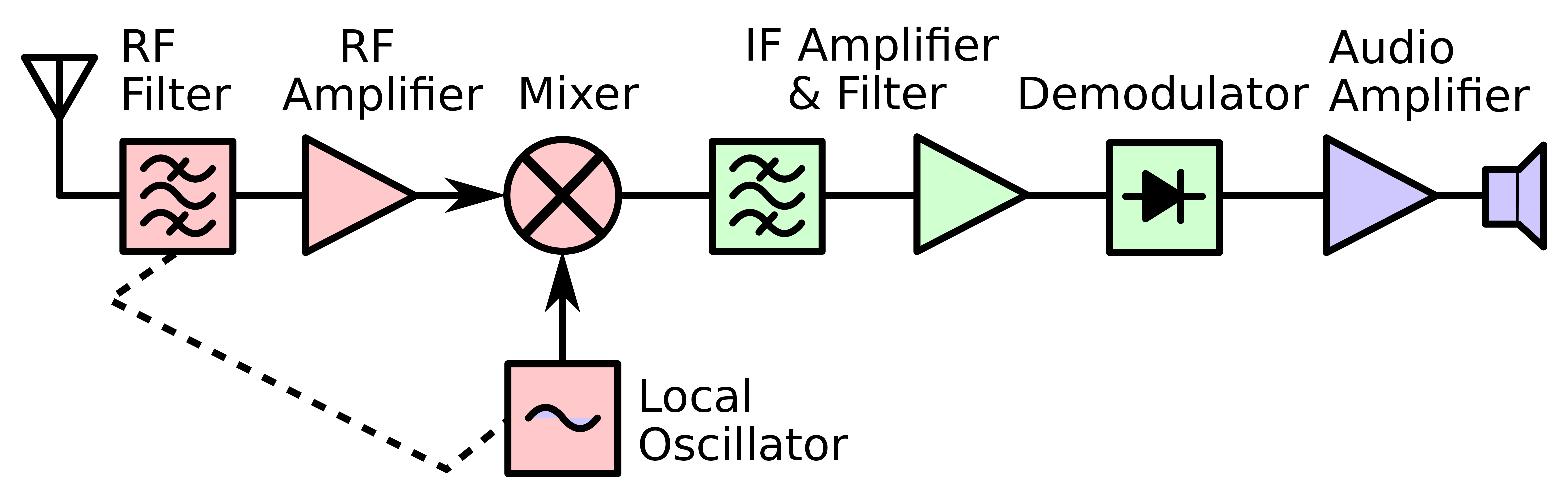
One of them was the superheterodyne receiver, which multiplies the receiving signal with a local oscillator signal as it can be seen in Figure 50. Thereby, the lower resulting frequency is often called intermediate frequency (ωIF or fIF ).
The bandpass at the beginning of Figure 50 is used to suppress out-of-band signals. Furthermore, an amplifier is present which might cause issues when the signal is to strong since the amplifier is then not working in its linear region any more. The amplifier is needed because of the mixer, since the mixer has an insertion loss. The IF bandpass filter is used filter out unwanted frequencies and to select the correct channel. To change the receiving
frequency one has to changes the oscillator frequency, since the second bandpass is normally constant.
So the RF bandpass is used to do the band selection and remove the image frequency and the if bandpass selects the channel. Sometimes there are two RF filters (one before and one after the amplifier) this is done to keep the insertion loss quite low. ⇒ first filter is not very good, but has nearly no insertion loss second filter has more insertion loss, but signal was already amplified.
The different symbols mean the following:
To design a superheterodyne receiver, one must be familiar with the trigonometric identities especially with the product identities, which can be seen in Equation 69. From those one can then derive Equation 70.
| (69) |
| (70) |
Due to the properties derived in the formulas above, one could think it’s super easy to to get a RF signal to a lower one. The only issue one has is that the received signal is not ideal, one has always some noise on it and one can not create ideal bandpass filters. Which means when ωLO is chosen to small and the bandpass is to large the new signal on the frequency ωLO is overlapped by the image frequency (frequency which is mapped to the same fIF as
the fRF signal).
For example in Figure 51 when we choose fLO to be fLO1 the fRF and fIM1 produce the frequency fIF according to Equation 70. Due to that, one needs a bandpass filter as it can be seen in Figure 52. There the bandpass filter is not ideal and still some noise from fIM1 superimposes the signal on fIF . In Figure 51 and Figure 52 one also sees the smaller ωIF gets the better the bandpass must be. Furthermore one sees that the image frequency is given
by Equation 71.
| (71) |
A direct-conversion receiver (DCR), also known as homodyne, synchrodyne, or zero-IF receiver, is a radio receiver design that demodulates the incoming radio signal using synchronous detection driven by a local oscillator whose frequency is identical to, or very close to the carrier frequency of the intended signal. The benefit is that one does not have image frequencies and no need of huge analogue filters is needed. The drawback is the receiver topology is
more complicated. One needs to do a hilbert transform. Exactly 90 degree phase shift is required.
Direct multiplying the RF input signal is only possible when Equation 72 is fullfilled.
| (72) |
For example one has the signal (sin(x× 2) + sin(x× 2.1) - sin(x× 1.9)) and want to transform it with this mehtod, therefore one multiplies it with sin(2x) which results in the following: sin(2x)(sin(x× 2) + sin(x× 2.1) - sin(x× 1.9)) which results in the following:  (- cos(4.1x) - cos(4x) + cos(3.9x) + 1) from which one can see that some part of the signal is missing in the baseband. But when also doing the multiplication with a 90 degree pahse
shifted signal one also gets this part as it can be seen in the following: cos(2x)(sin(x × 2) + sin(x × 2.1) - sin(x × 1.9)) which is
(- cos(4.1x) - cos(4x) + cos(3.9x) + 1) from which one can see that some part of the signal is missing in the baseband. But when also doing the multiplication with a 90 degree pahse
shifted signal one also gets this part as it can be seen in the following: cos(2x)(sin(x × 2) + sin(x × 2.1) - sin(x × 1.9)) which is  (sin(4.1x) + sin(4x) - sin(3.9x) + 2 sin(0.1x))


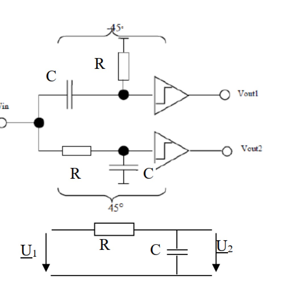
Show that a broadband 90∘ phase shifting can be realized using the circuit topology in Figure 53


What would be the amplitude characteristics without limiting amplifiers?


90∘ phase shifter
Find an almost ideal 90∘ phase shifter topology consisting of a ’divide by 2’ counter and an oscillator.
DC offset in zero-IF receivers/ self-mixing process Assume that the LO power of a zero-IF receiver is given by PLO=0dBm. All impedances are Zo=50 Ω. The isolation between the mixer’s LO port and the LNA’s input port is 60dB (when connected at the antenna). The amplification of the combination of LNA and Mixer is 30dB.
Calculate the resulting voltage at the mixer’s output. Compare this voltage with the the rms value of the voltage resulting from an RF signal of -80dBm at the antenna footpoint.
Note: The figure of 30dB isolation between LO and RF port is with connected antenna i.e. the coupled LO power is divided by 2, one half travelling towards the antenna, the other half travelling towards the LNA input port.
DC power at mixer’s output: (0-30-30+30) dBm = -30 dBm Rightarrow 7mV @ 50Ω RF power at mixer’s output: (-80+30) dBm = -50 dBm Rightarrow 0.7mV rms @ 50Ω
the DC offset voltage is 10x higher as a reasonably strong RF input signal!
Even-order distortion in zero-IF receivers
Show that zero-IF receivers are susceptible(anf��llig) to even-order distortions.
Second order nonlinearity: y = x2
![x(t) := x1(t) + x2(t)
x1(t) = cos(ω1 ⋅ t) x2(t) = cos(ω2 ⋅ t)
⇒ y (t) = [cos(ω ⋅ t) + cos (ω ⋅ t)]2 = cos2(ω ⋅ t) + cos2 (ω ⋅ t) + 2 ⋅ cos(ω ⋅ t) ⋅ co
2 12 2 1 2 1 2
cos (ω1 ⋅ t) + cos (ω2 ⋅ t) + {cos [(ω1 + ω2 ) ⋅ t] + cos [(ω1 - ω2 ) ⋅ t]}](main2_for_html372x.svg)
If ω1 ≈ ω2 then the component  is a signal near DC, which could interfere with the downconverted wanted signal.
Choice of Receiver Topology
Give some examples how the choice of receiver topology could be influenced by circuit design, economical or other issues.
Superheterodyne Receiver
Discuss the advantage/disadvantage of having the bandpass before and after the amplifier in a superhet receiver with respect to receiver performance:
When the amplifier is before the filter the total noise figure will be improved, but the large signal behaviour becomes worse. Therefore, when one wants high sensitivity the amplifier must be at the beginning, whereas when one wants good large signal behaviour the amplifier must come after the filter.
Superheterodyne Receiver
A receiver has to be designed covering a receiving frequency range between 118...136 MHz. Determine the lowest possible intermediate frequency in order to be able to remove any image frequency by an RF filter in front of the mixer stage. Determine the local oscillator’s frequeny range for this case for the two possibilities fRF < fLOf and fRF < FLOf. Considering the result of b), which problem arises if an IF near the minimum IF is used? What would
be the minimum value of the IF to circumvent the problem in c)? Discuss advantages and disadvantages to select the LO frequency above or below the receiving frequency
 of the bandwidth of the signal which is fIF >
  ⋅ (fRFmax - fRFmax) = 9MHz.
 furthermore, the sign is minus for the case where fLF < fRF due to that and the fact that fRF - fLF = 9MHz must always be true fLF has a range from 109-127MHz. For the case where fLF > fRF the sign is opposite and therefore in the range 127MHz-145MHz.
To avoid the second problem in c):

fLO < fRF
Advantages:
Disadvantages:
fLO > fRF vice versa
Dual-IF topology with image-signal rejection
A given dual-IF topology (see above figure) has the following specifications:
fRF = 87.5MHz...108 MHz
Bandwidth of the received signal: B=180kHz
First IF at fIF1=10.7 MHz
Second IF at fIF2=455 kHz
fLO1 < fRF
Determine all spurious signals which could occur due to the selection of this set of intermediate frequencies if the RF input frequency is given by fRF = 90.7 MHz. Why is Filter 2 in Figure 56 needed? What is the maximum bandwidth of Filter 2 in Figure 56 to fulfil its function (see b))?
2 possible cases for fLO2 :
Other mixing products

Need of Filter 2

Designing sharp filters for high frequencies in CMOS technology, which is often used, is quite difficult. Due to that one came up with different receiver technologies to be able to implement those filters at lower frequencies. To do that one ore more local oscillators are needed which consume quite a lot of energy. Therefore nowadays, one tries to prevent having local oscillators when possible. Nevertheless, it was often used and is still used in some applications. Therefore one has a look at them in this chapter.
Problem is that when signal is not symmetric it is not working. A solution would be to multiplie it with a complex signal.
| (73) |
This is the idea of the zero-if approach. The issue is when one has a little phase shift then one gets some image. One issue of this approach is the dc offset. When something is near the antenna the antenna has a different impedance. From the mixer some signal goes to the antenna with the ωLO frequency. When the antenna is not matched the signal comes back the amount of the signal that comes back is dependent on the environment. Today one solves this problem by leaving always the carrier in the middle at the frequency of zero.
It is difficult to have a 90 degree phase shift for a whole frequency band. The image rejection ratio can be callculated with Equation 74 where the variables mean the following:
δG = amplitude error
δφ = phase error
| (74) |
An analog bandpass signal x(t) can be fully reconstructed if it’s sampled with a frequency of more than two times the bandwidth of x(t)
Sampled signal

![[ ]
1 ∑∞ ( n )
Spectrum of the sampled signal Xa (f) = X (f) * -- δ f - --
T n=- ∞ T](main2_for_html384x.svg)

The idea is to get a digital downconversion instead of a analog one, due to sampling theorem. The problem is that one has mirror from the left side, therefore it would be nice if one can remove it. Analytic signal has only positive frequency components, is not anymore a real time signal, since a real signal has always a positive and negative part.
The frequency response of the channel is given by H(t).
| (75) |
Important wave progpagations modes
Image Reject Mixers: Calculate the image rejection ratio at a given phase error of 3∘ and an amplitude error of 2 dB
According to Equation 74 the following holds:

where δG = amplitude error and δφ = phase error, therefore  = 10
= 10 - 1 = 0.259.

The calculation of the power density SR at the receiver at a given distance d can be done according to Equation 76, where P is the power and GT the antenna gain.
| (76) |
The pointing vector can be calculated according to Equation 77
| (77) |
The field wave impedance can be calculated according to Equation 78
| (78) |
The Electrical field strength (rms) can be calculated according to Equation 79, which as the combination of Equation 78, Equation 77 and Equation 76.
| (79) |
The equivalent absorption area of a receiving antenna is given by Equation 80
| (80) |
| (81) |
Equation 82 Shows the free space loss:
| (82) |
Where λ =  .
.
| (83) |
Correction terms
Correction term for small and medium-sized cities:

Correction term for metropolises:
![{
8.29 ⋅ [log (1.54 ⋅ hMS-)]2- 1.1 f ≤ 200MHz
a(hMS ) = [ ( hm )]22
3.2 ⋅ log 11.75 ⋅-MmS- - 4.97 f ≥ 400MHz](main2_for_html401x.svg)
Correction term for sub-urban areas:
![[ f ]2
LHs [dB ] = LHu - 2 ⋅ log ------- - 5.4
28MHz](main2_for_html402x.svg)
Correction term for rural areas:
![[ ]2
--f--- --f---
LHr [dB ] = LHu - 4.78 ⋅ logM Hz + 18.33 ⋅ log M Hz - 40.94](main2_for_html403x.svg)
Due to variations of air temperature/pressure/humidity, the refraction index varies with height above ground.

The Doppler frequency is described with Equation 84
| (84) |
The maximum Doppler frequency fm is given by
| (85) |
Coherence Time: measure for the time period in which the channel properties remain approximately constant.
| (86) |
Bd = Doppler spread bandwidth
Coherence bandwidth: measure for the bandwidth, in which the channel properties remain highly correlated.
| (87) |
Tm = delay spread
⇒ all frequency component within Bcb will be almost equally attenuated.
Two-ray-model A base station transceiver transmits a GSM signal on a channel within the frequency range of f = 935,2MHz...935.4MHz. A mobile station (MS) is connected to this base station (BS). Let us assume that there is a line-of sight condition between them. Imagine further that there is a mountain chain parallel to the line-of-sight connection at a distance of h=2km, which partially reflects incident radio signals. Let us assume further:
Determine the radio channel’s amplitude response between the BS and the MS for the given GSM-channel (i.e. between 935,2 MHz ... 935,4 MHz)
According to Equation 63 the following holds:

Due to that the received signal is

and


And the Amplitude spectrum of the graph in the range from 935,2MHz...935.4MHz looks like in Figure 59
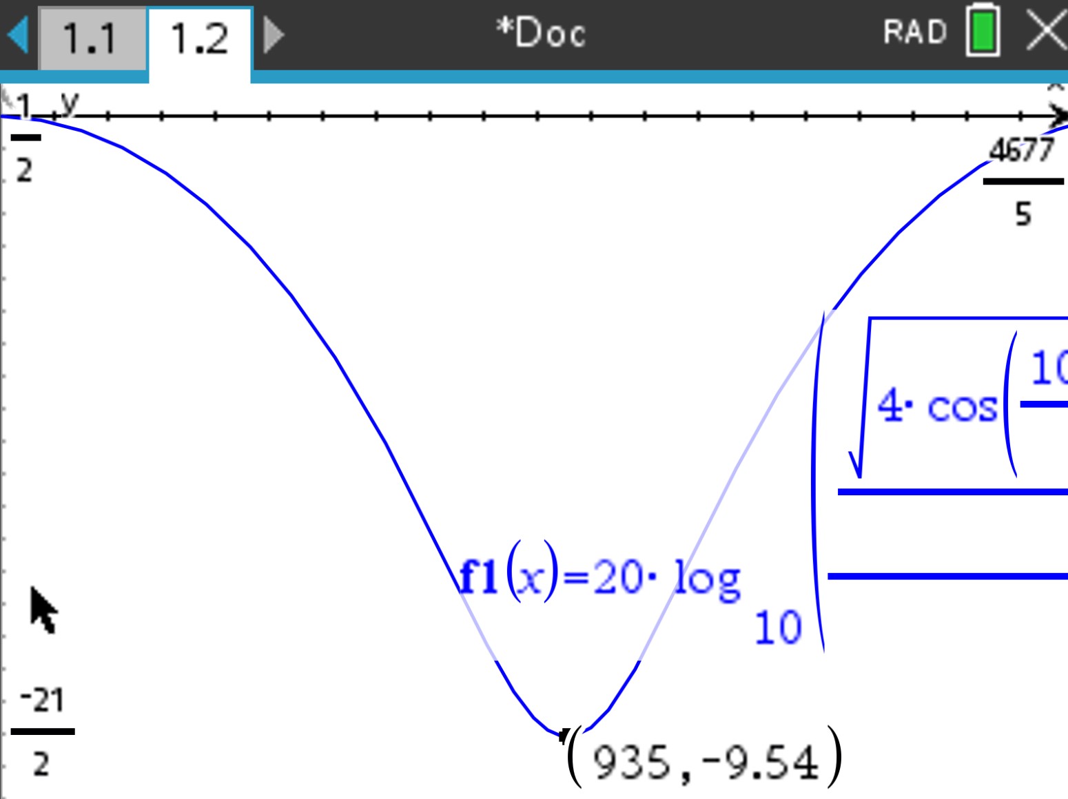
 )2 = 35.53 × 10⁹ and in dB: 10 log
10(35.53 × 10⁹) = 105.512dB
)2 = 35.53 × 10⁹ and in dB: 10 log
10(35.53 × 10⁹) = 105.512dB
 =
=  = 24.4949 × 10⁻³ V m-1
Determine the path loss in urban environment using the Okumura-Hata model for the following scenario:
According to Equation 83 one knows that
![( )
--f--- hBS- hBS- -d--
LHu [dB ] = 69.55 + 26.16 ⋅ log M Hz - 13.82 ⋅ log m - a◟(hM◝S◜-)◞ + 44.9 - 6.55 log m ⋅ log km
0 for urban
= 69.55 + 26.16 ⋅ log(900 ) - 13.82 ⋅ log(50m ) + (44.9 - 6.55 log (50m )) ⋅ log 5
= 146.959dB--](main2_for_html416x.svg)
Same scenario, but for rural environment
![L [dB ] = 146.959dB - 4.78 ⋅ [log (900 )]2 + 18.33 ⋅ log (900 ) - 40.94 = 118.452dB
Hr -----------](main2_for_html417x.svg)
Time-variant channel modelling I
 =
=  = 0.1 ms. ==� The delay line model consists of 10 taps where only the first and the last have (time-varying coefficients)
 = 1000 Hz. Within this bandwidth all frequency components of a signal are modified in a similar way, e.g. all frequency components within Bc could be simultaneously attenuated.
Time-variant channel modelling II
Exam: Bring laptop with to the exam, submission is online, when we write on papaer, we have to scan in programms on the computer are not allowed but local pdfs are.
| (88) |
Ein Bernoulli-Experiment mit den beiden sich gegenseitig ausschliessenden Ergebnissen (Ereignissen) A und Ā werde n-mal nacheinander ausgefuehrt (sog. mehrstufiges Bernoulli-Experiment vom Umfang n ). Dann genuegt die diskrete Zufallsvariable

der sog. Binomialverteilung mit der Wahrscheinlichkeitsfunktion
| (89) |
und der zugehoerigen Verteilungsfunktion

(fuer x < 0 ist F(x) = 0 ). n und p sind dabei die Parameter der Verteilung. Die Kennwerte oder Masszahlen der Binomialverteilung lauten:
 =
= 
Dabei bedeuten:
| Degrees | 0∘ | 30∘ | 45∘ | 60∘ | 90∘ | ||
| Radians | 0 |  |  |  |  |
||
| sinθ | 0 |  |  |  | 1 | ||
| cosθ | 1 |  |  |  | 0 | ||
| tanθ | 0 |  | 1 |  | |||
| cot x | =  | ||
| csc x | =  | ||
| sec x | =  |
| sin(-x) | = - sin x | ||
| cos(-x) | = cos x | ||
| tan(-x) | = - tan x |
| sin 2x + cos 2x | = 1 | ||
| 1 + tan 2x | = sec 2x | ||
| 1 + cot 2x | = csc 2x |
sin( - x) - x) | = cos x | ||
cos( - x) - x) | = sin x | ||
tan( - x) - x) | = cot x | ||
cot( - x) - x) | = tan x | ||
sec( - x) - x) | = csc x | ||
csc( - x) - x) | = sec x |
| sin(x + y) | = sin x cos y + cos x sin y | ||
| sin(x - y) | = sin x cos y - cos x sin y | ||
| cos(x + y) | = cos x cos y - sin x sin y | ||
| cos(x - y) | = cos x cos y + sin x sin y | ||
| tan(x + y) | =  | ||
| tan(x - y) | =  |
| sin(2x) | = 2 sin x cos x | ||
| cos(2x) | = cos 2x - sin 2x | ||
| = 2 cos 2x - 1 | |||
| = 1 - 2 sin 2x | |||
| tan(2x) | =  |
sin  | = � | ||
cos  | = � | ||
tan  | =  | ||
=  |
| sin 2x | =  | ||
| cos 2x | =  | ||
| tan 2x | =  |
| sin x sin y | =   cos(x - y) - cos(x + y) cos(x - y) - cos(x + y)![]](main2_for_html463x.svg) | ||
| cos x cos y | =   cos(x - y) + cos(x + y) cos(x - y) + cos(x + y)![]](main2_for_html466x.svg) | ||
| sin x cos y | =   sin(x + y) + sin(x - y) sin(x + y) + sin(x - y)![]](main2_for_html469x.svg) | ||
| tan x tan y | =  | ||
| tan x cot y | =  |
| sin x + sin y | = 2 sin    cos cos    | ||
| sin x - sin y | = 2 cos    sin sin    | ||
| cos x + cos y | = 2 cos    cos cos    | ||
| cos x - cos y | = -2 sin    sin sin    | ||
| tan x + tan y | =  | ||
| tan x - tan y | =  | ||
Why  see the following video
| Real-/Imaginary part: | Re{x} = xR =  ![*
[x + x ]](main2_for_html500x.svg) | Im{x} = x
I =  ![*
[x - x ]](main2_for_html502x.svg) |
| even/odd part: | xg(t) =  [x(t) + x(-t)] [x(t) + x(-t)] | xu(t) =  [x(t) - x(-t)] [x(t) - x(-t)] |
| conj. even/odd part: | xg*(t) =  ![[x(t) + x*(- t)]](main2_for_html506x.svg) | x
u*(t) =  ![[x (t) - x*(- t)]](main2_for_html508x.svg) |
| aperiodisch | periodisch | |
| diskret: | x[n] * y[n] = ∑ i=-∞∞x[i] ⋅ y[n - i] | x[n] ⊛ y[n] = ∑ i=n0n0+Np-1x[i] ⋅ y[n - i] |
| kontinuierlich: | x(t) * y(t) = ∫ -∞∞x(τ) ⋅ y(t - τ)dτ | x(t) ⊛ y(t) = ∫ t0t0+Tpx(τ) ⋅ y(t - τ)dτ |
| diskret: | Ex(d) = ∑
k=-∞∞|x[k]|2 = T ∫
-1∕2T 1∕2T |X(f)|2df =  ∫
-ππ|X(Ω)|2dΩ ∫
-ππ|X(Ω)|2dΩ |
| kontinuierlich: | Ex(k) = ∫
-∞∞|x(t)|2dt = ∫
-∞∞|X(f)|2df =  ∫
-∞∞|X(jω)|2dω = T ⋅ E
x(d) ∫
-∞∞|X(jω)|2dω = T ⋅ E
x(d) |
| diskret: | Px(d) =  ∑
k=0Np-1|x[k]|2 = ∑
n=0Np-1 ∑
k=0Np-1|x[k]|2 = ∑
n=0Np-1 2 = 2 =  ∑
n=0Np-1|X[n]|2 ∑
n=0Np-1|X[n]|2 |
| kontinuierlich: | Px(k) =  ∫
-Tp∕2Tp∕2|x(t)|2dt = ∑
n=-∞∞ ∫
-Tp∕2Tp∕2|x(t)|2dt = ∑
n=-∞∞ 2 = P
x(d) 2 = P
x(d) |
| Impulskamm: | WT (t) = ∑
n=-∞∞δ(t - nT) =  W W |
| periodische Impulsfolge: | UN[k] = ∑ n=-∞∞δ[k - nN] |
| zweiseitig: | einseitig: |
| X(z) = ∑ k=-∞∞x[k]z-k | X(z) = ∑ k=0∞x[k]z-k |
Konvergenzgebiet  : a < |z| < b : a < |z| < b | Konvergenzgebiet : |z| > a |
x[k] =  ∮ ∮
 X(z)zk-1dz = ∑
αi∈ X(z)zk-1dz = ∑
αi∈ Res Res 
 : pos. orientierte Kurve in . : pos. orientierte Kurve in .  : Menge aller von umschlossenen Pole. : Menge aller von umschlossenen Pole. |
| Zeitbereich | Bildbereich | Konvergenz | |
| Linearit��t | c1x1[k] + c2x2[k] | c1X1(z) + c2X2(z) | x1 ∩x2 |
| Faltung | x[k] * y[k] | X(z) ⋅ Y (z) | x ∩y |
| Verschiebung | x![[k - k0]](main2_for_html520x.svg) | z-k0X(z) |
x |
| D��mpfung | ak ⋅ x[k] | X | |a|⋅x |
| lineare Gewichtung | k ⋅ x[k] | -z ⋅ X(z) X(z) | x |
| konj. komplexes Signal | x*[k] | X* |
x |
| Zeitinversion | x[-k] | X | 1∕x |
| diskrete Ableitung | x[k] - x[k - 1] | X(z) ⋅ | x |
| diskrete Integration | ∑ i=∞kx[i] | X(z) ⋅ | x ∩{|z| > 1} |
| periodische Fortsetzung | ∑
i=0∞x![[k - iN ]
p](main2_for_html527x.svg) | X(z) ⋅ | x ∩{|z| > 1} |
| Upsampling | x![[ k-]
N](main2_for_html529x.svg) | X |  x
x |
![|---------------------|------------------|----------------------------∑k---1---------------------------|
| Verschiebung links |x [k + k0],k0 > 0 | zk0X (z) - i0=0 x[i]zk0-i |
|---------------------|------------------|------------------k--------∑---1---------k--i----------------|
|-Verschiebung-rechts-|x-[k---k0],k0->-0-------------------z--0X-(z) +---i=--k0 x[i]z--0------------------|
| | |
|-Anfangswertsatz-----|-----------------x[0] =-limz→-∞-X-(z),-falls-Grenzwert--existiert-----------------|
| | |
--Endwertsatz----------limk-→-∞-x[k] =-limz→1-(z --1)X-(z),-falls-X(z)-nur-Pole-mit|z| <-1-oder-bei-z-=-1-](main2_for_html532x.svg)
Die Partialbruchzerlegung von X(z) =  f��hrt auf die Form:
X(z) = ∑
i≥1gi ⋅ zi + ∑
i + ∑
i ∑
l=1mi + ∑
i ∑
l=1mi , gi, αi, αi, ri, ri,l ∈ ℂ, , gi, αi, αi, ri, ri,l ∈ ℂ, |
welche f��r : |z| > r0 mit den Korrespondenzen 2, 5, 6 und 12 gliedweise zur��cktransformiert werden kann.
| Nr. | x[k] | X(z) | |
| 1 | δ[k] | 1 | z ∈ ℂ |
| 2 | δ![[k - k0]](main2_for_html536x.svg) | z-k0 | 0 < |z| < ∞ |
| 3 | ε[k] |  | |z| > 1 |
| 4 | k ⋅ ε[k] |  | |z| > 1 |
| 5 | ak ⋅ ε[k] |  | |z| > |a| |
| 6 |  ak-m ⋅ ε[k] ak-m ⋅ ε[k] |  | |z| > |a| |
| 7 | sin  ⋅ ε[k] ⋅ ε[k] |  | |z| > 1 |
| 8 | cos  ⋅ ε[k] ⋅ ε[k] | ![zz2⋅-[z2-zc⋅coos(s(ΩΩ00))+]1-](main2_for_html545x.svg) | |z| > 1 |
| 9 | ak ⋅ ε[-k - 1] | - | |a| < |a| |
| 10 | a|k|, |a| < 1 |  |
|
| 11 |  ⋅ ε[k] ⋅ ε[k] | e
| |z| <  |
Spezielle Korrespondenzen zur R��cktransformation konj. komplexer Polpaare
| 12 | 2|r∥α|k cos(∢α ⋅ k + ∢r) ⋅ ε[k] |  + +  | |z| > α |
| 13 | ak ⋅ ⋅ ε[k] ⋅ ε[k] |  , c > , c >  | |z| >  |
a =  , Ω
0 = arccos , Ω
0 = arccos  , φ0 = arctan , φ0 = arctan  | |||
| zweiseitig: | einseitig: |
| X(s) = ∫ -∞∞x(t)e-stdt | X(s) = ∫ 0-∞x(t)e-stdt |
| Konvergenzgebiet : a < Re{s} < b | Konvergenzgebiet : Re{s} > a |
| Zeitbereich | Bildbereich | Konvergenz | |
| Linearit��t | c1x1(t) + c2x2(t) | c1X1(s) + c2X2(s) | x1 ∩x2 |
| Faltung | x(t) * y(t) | X(s) ⋅ Y (s) | x ∩y |
| Verschiebung | x | e-st0 ⋅ X(s) |
x |
| D��mpfung | eat ⋅ x(t) | X(s - a) |
x + Re{a} |
| lineare Gewichtung | t ⋅ x(t) | - X(s) X(s) | x |
| Differentiation |  x(t) x(t) | s ⋅ X(s) | x |
| Integration | ∫ -∞tx(τ)dτ |  ⋅ X(s) ⋅ X(s) | x ∩{Re{s} > 0} |
| Skalierung | x(at) |  ⋅ X ⋅ X | a ⋅x |
| konj. komplexes Signal | x*(t) | X*(s*) |
x |
![|---------------------|-----------------|---------[--------∫--------------]------|
| Verschiebung links |x (t + t0),t0 > 0| est0 X (s) - t0- x (t) ⋅ e-stdt |
|---------------------|-----------------|---------[--------∫0--------------]-----|
| Verschiebung rechts |x (t - t0),t0 > 0| e-st0 X (s ) + 0 x (t) ⋅ e-stdt |
|---------------------|-----------------|--------------------t0------------------|
| Differentiation | -dx(t) | s ⋅ X (s) - x(0- ) |
|---------------------|-----dt---------------------------------------------------|
| Anfangswertsatz | x (0+) = lims→ ∞ s ⋅ X (s ), falls x (0+) existiert |
|---------------------|----------------------------------------------------------|
--Endwertsatz----------limt-→∞-x-(t)-=-lims→0-s-⋅ X-(s),-falls-limt→-∞-x(t)-existiert--](main2_for_html566x.svg)


kann f��r : Re{s} > a0 mit den Korrespondenzen 1, 4, 5 und 10 gliedweise zur��cktransformiert werden.
| Nr. | x(t) | X(s) | |
| 1 | δ(t) | 1 | s ∈ ℂ |
| 2 | ε(t) |  | Re{s} > 0 |
| 3 | ρ(t) = t ⋅ ε(t) |  | Re{s} > 0 |
| 4 | eat ⋅ ε(t) |  | Re{s} > Re{a} |
| 5 |  eat ⋅ ε(t) eat ⋅ ε(t) |  | Re{s} > Re{a} |
| 6 | sin  ⋅ ε(t) ⋅ ε(t) |  | Re{s} > 0 |
| 7 | cos  ⋅ ε(t) ⋅ ε(t) |  | Re{s} > 0 |
| 8 | sin  ⋅ ε(t) ⋅ ε(t) |  | Re{s} > 0 |
| 9 | δ | e-st0 | s ∈ ℂ |
| 10 | 2|r|eRe{α}t cos(Im{α}t + ∢r)ε(t) |  + +  | Re{s} > Re{α} |
| 11 | eat ⋅ ⋅ ε(t) ⋅ ε(t) |  , c > , c >  | Re{s} >  |
a =  , ω0 = , ω0 =  , φ0 = arctan , φ0 = arctan  | |||
| Definition: | R��cktransformation: |
| X(f) = ∫ -∞∞x(t) ⋅ e-j2πftdt | x(t) = ∫ -∞∞X(f) ⋅ ej2πftdf |
Definition ��ber die Kreisfrequenz ω = 2πf :
X(jω) = ∫
-∞∞x(t) ⋅ e-jωtdt x(t) =  ∫
-∞∞X(jω) ⋅ ejωtdω
∫
-∞∞X(jω) ⋅ ejωtdω
![|-------------------------|---Zeitbereich---|-----------------Frequenzbereich------------------|
| | | | |
|-Linearity---------------|c1x1(t)-+-c2x2(t)|--c1X1-(f)-+-c2X2(f-)--|--c1X1-(jω)-+-c2X2-(j-ω)---|
| | | | |
|-Faltung-----------------|----x(t) *-y(t)---|------X-(f) ⋅ Y-(f)----|------X-(jω) ⋅-Y(jω-)-----|
| Multiplikation | x(t) ⋅ y(t) | X (f ) * Y(f ) | -1X (jω ) * Y (jω) |
|-------------------------|-----------------|-----------------------|----2π--------------------|
| Verschiebung | x (t - t0) | X (f ) ⋅ e-j2πft0 | X (jω) ⋅ e-jωt0 |
|-------------------------|-----------------|-----------------------|--------------------------|
| Modulation | ej2πf0t ⋅ x (t) | X (f - f0) | X (j [ω - ω0]) |
|-------------------------|-----------------|-----------------------|--------------------------|
| lineare Gewichtung | t ⋅ x(t) | - 1j2π-ddfX (f) | - d(djω)X (jω ) |
|-------------------------|------d----------|-----------------------|--------------------------|
|-Di-fferentiation----------|------dtx-(t)------|------j2πf-⋅ X-(f)-----|-------jω-⋅-X-(j-ω)--------|
| | ∫t | -1-- 1 | 1- |
|-Integration-------------|-----∞-x-(τ-)dτ---|-j2πfX-(f-) +-2X-(0)δ(f-)--jωX-(jω)-+-πX-(0)δ(f-)--|
| | | 1- (f) | -1 (jω-) |
|-Skalierung--------------|------x(at)------|-------|a| ⋅ X-a--------|-----|a|-⋅ X--a--δ(ω)------|
| Zeitinversion | x(- t) | X (- f) | X (- jω ) |
|-------------------------|-----------------|-----------------------|--------------------------|
| konj. komplex | x*(t) | X *(- f) | X *(- jω) |
|-------------------------|-----------------|-----------------------|--------------------------|
| Real part | xR(t) | Xg *(f) | Xg*(jω ) |
|-------------------------|-----------------|-----------------------|--------------------------|
|-Imaginary--part---------|------jxI(t)------|--------Xu-*(f)--------|---------Xu*(jω-)---------|
| | | | |
|-duality-----------------|---X-(t)[X-(jt)]-----------x-(- f-)----------------2πx-(--ω)---------|
| |∫ ∞ * ∫∞ * -1 ∫∞ * |
--Parsevalsches-Theorem-------∞-x(t) ⋅ y-(t)dt-=--∞-X-(f-) ⋅ Y-(f)df-=-2π--∞-X-(jω-) ⋅ Y-(jω)dω-](main2_for_html591x.svg)
![--Nr.------------x-(t)----------------------X-(f-)----------------------X-(jω)------------
|------|-----------------------|---------------------------|---------------------------|
| 1 | δ(t) | 1 | 1 |
|------|-----------------------|---------------------------|---------------------------|
|--2---|-----------1-----------|-----------δ(f)------------|----------2πδ(ω)-----------|
| | | 1-- | -2π- |
|--3---|--------UT-(t)---------|---------|T|IH-1T (f)--------|--------|T|U-2πT-(ω-)---------|
| | | 1 --1- | -1 |
|--4---|---------ε(t)----------|-------2δ(f-) +-j2πf-------|--------πδ(ω)-+-jω---------|
| 5 | sgn (t) | -1- | -2 |
|------|-----------------------|------------jπf------------|------------jω-------------|
| 6 | -1 | - j sgn (f) | - j sgn (ω ) |
|------|----(--)--πt-----------|---------------------------|--------------(---)--------|
| 7 |rect Tt (T = width )| |T| ⋅ si(πT f) | |T| ⋅ si T2ω |
|------|----------(--t)--------|---------------------------|--------------(T---)-------|
|--8---|--------si-πT----------|-------|T-| ⋅ rect(Tf-)-----|------|T-| ⋅ rect-2π-ω-------|
| | (t-) | 2 | 2(T- ) |
|--9---|--------Λ---T----------|-------|T-| ⋅ si-(πT-f-)-----|-------|T-| ⋅ si-2-ω--------|
| | 2( t) | | (T-- ) |
|-10---|-------si--π-T---------|--------|T-| ⋅ Λ-(Tf-)------|-------|T-| ⋅ Λ-2π-ω---------|
| 11 | ej2πf0t | δ (f - f ) | 2πδ (ω - ω ) |
|------|-----------------------|----------------0----------|-----------------0---------|
| 12 | cos(2πf0t ) | 1 [δ (f + f0) + δ (f - f0)]|π [δ(ω + ω0 ) + δ (ω - ω0)]|
|------|-----------------------|-2-------------------------|---------------------------|
| 13 | sin(2πf0t) | 12j [δ(f + f0) - δ(f - f0)]|πj [δ (ω + ω0) - δ(ω - ω0 )]|
|------|------------22---------|---------√----π2f2----------|---------√-----ω2----------|
| 14 | e -at | -πa e- a2 | -aπe-4a2 |
|------|------------|t|---------|------------2T-------------|------------2T-------------|
--15-------------e--T--------------------1+(2πTf)2---------------------1+(T-ω)2------------](main2_for_html592x.svg)
Where


![y(n) = -1 [x(n ) + x (n - 1) + x (n - 2) + x (n - 3) + ...+ x(n - D + 1)]
D](main2_for_html31x.svg)
![1 [ ]
Y (z) = -- X (z) + X (z )z -1 + X (z )z -2 + ...+ X (z)z-D+1
D](main2_for_html32x.svg)
![Y (z) 1 [ ] 1 D∑ -1
HMA (z) = ----- = -- 1 + z- 1 + z- 2 + ...+ z-D+1 = -- z- n
X (z) D D n=0](main2_for_html33x.svg)
![1-
y(n) = D [x(n) - x(n - D )] + y (n - 1)](main2_for_html34x.svg)


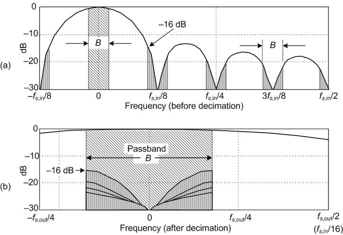
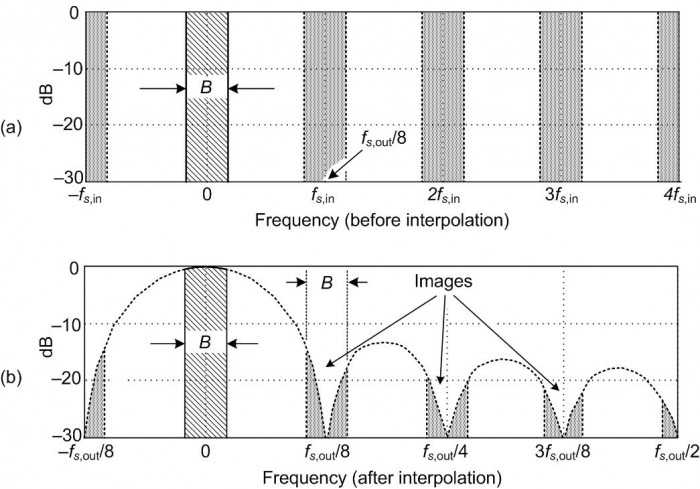


![---111
yzww+zw+zw+ˆsw[0123[nine]+neDr ] filter with M=4](main2_for_html122x.svg)
![∑
s+nˆsy[n[[n[]nMin]=+]0wDi] ⋅ y [n - i]](main2_for_html123x.svg)
![s+αzx+nyzww+ˆsw[n-[[[n-[ni]1nn1e]]]+neDr] filter
01](main2_for_html135x.svg)
![*
w [k + 1] = w [k] + μ ⋅ e[k] ⋅ x [k]](main2_for_html158x.svg)
![-1
w = w + ----R-k-1y-[k]-----(d[k] - xT[k]w )
RLS,k RLS,k- 1 xT[k]R -k1-1y[k] + 1 RLS,k- 1](main2_for_html168x.svg)


![xB+zAxC+vyx[-[[[kk1kkk+]]]]1](main2_for_html179x.svg)
![x+z1x+vyx[-[[[k1kkk]]]]
2k+1](main2_for_html180x.svg)
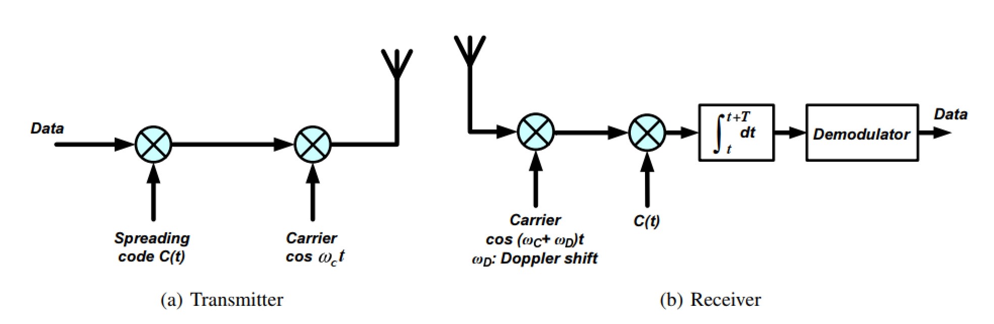

![H1 = [1[], ]
1 1
H2 = 1 - 1 ,
⌊ ⌋
1 1 1 1
|| 1 - 1 1 - 1 ||
H4 = ⌈ 1 1 - 1 - 1 ⌉
1 - 1 - 1 1
[ ]
H2k-1 H2k-1
H2k = H2k-1 - H2k-1 = H2 ⊗ H2k-1](main2_for_html206x.svg)
![⌊ ⌋ ⌊ ⌋
1 ⋅ 0 1 ⋅ 5 2 ⋅ 0 2 ⋅ 5 0 5 0 10
[ 1 2 ] [ 0 5 ] | 1 ⋅ 6 1 ⋅ 7 2 ⋅ 6 2 ⋅ 7 | | 6 7 12 14 |
⊗ - |⌈ |⌉ - |⌈ |⌉
3 4 6 7 3 ⋅ 0 3 ⋅ 5 4 ⋅ 0 4 ⋅ 5 0 15 0 20
3 ⋅ 6 3 ⋅ 7 4 ⋅ 6 4 ⋅ 7 18 21 24 28](main2_for_html207x.svg)
![H ⋅ HT = [ 1 - 1 1 - 1 1 - 1 1 - 1 ] ⋅ [ 1 - 1 - 1 1 - 1 1 1 - 1 ]T
82 88
= 1 + 1 - 1 - 1 - 1 - 1 + 1 + 1 = 0.](main2_for_html209x.svg)


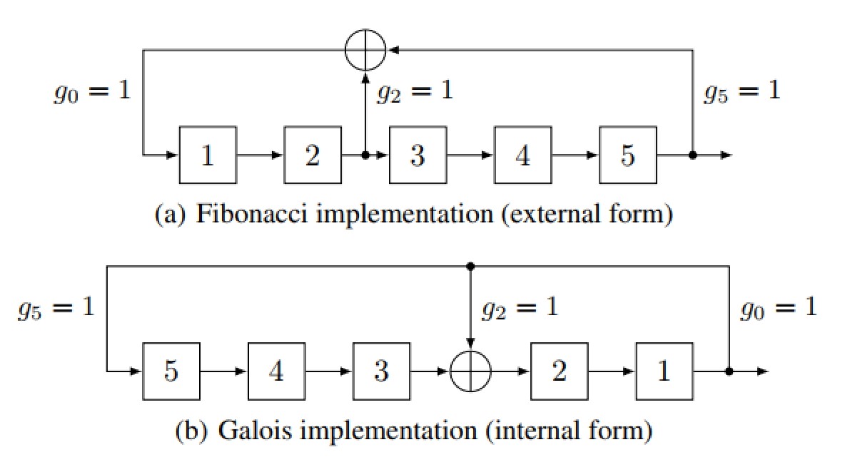


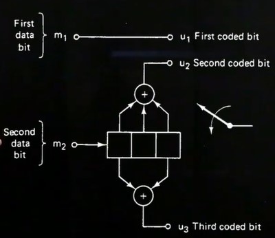
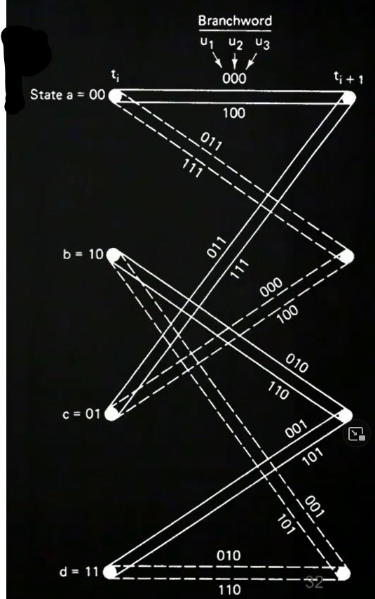
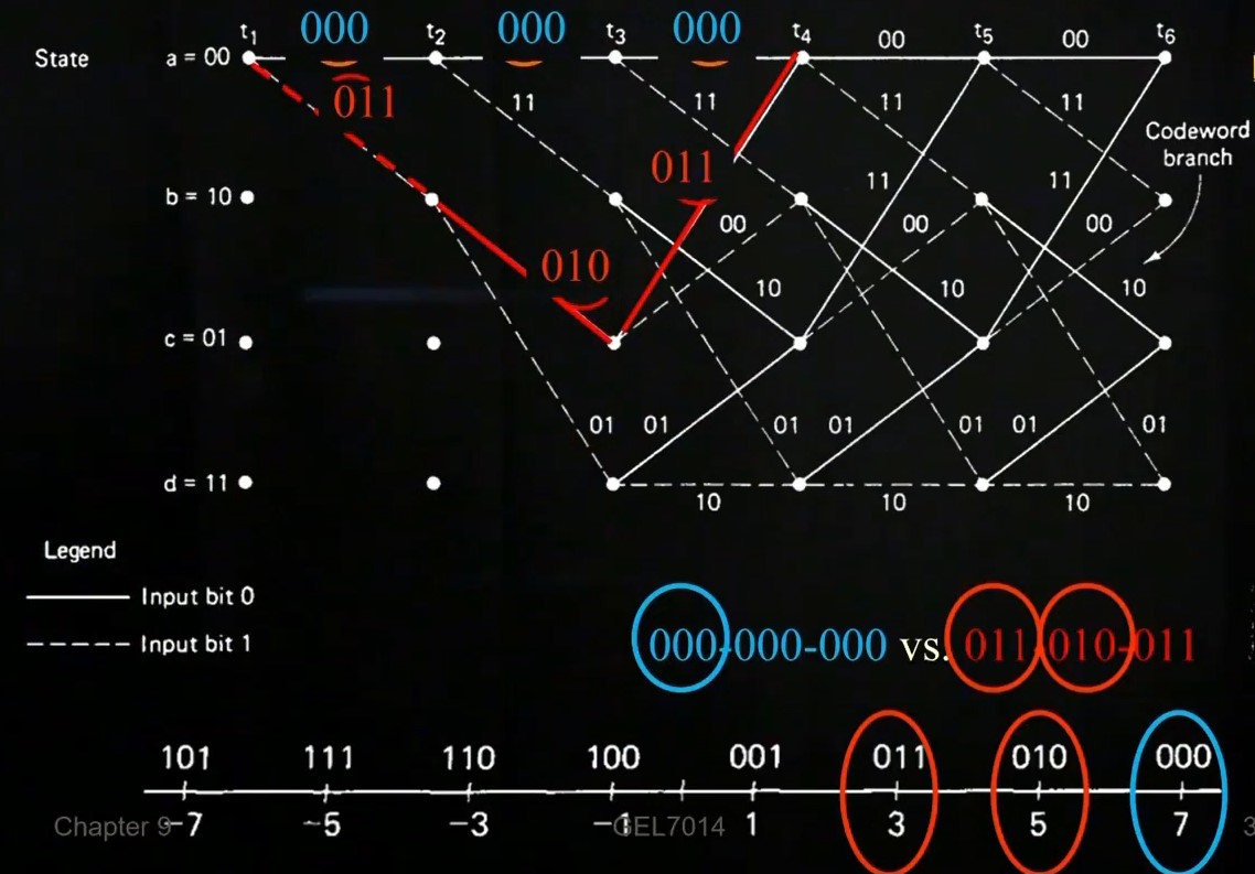
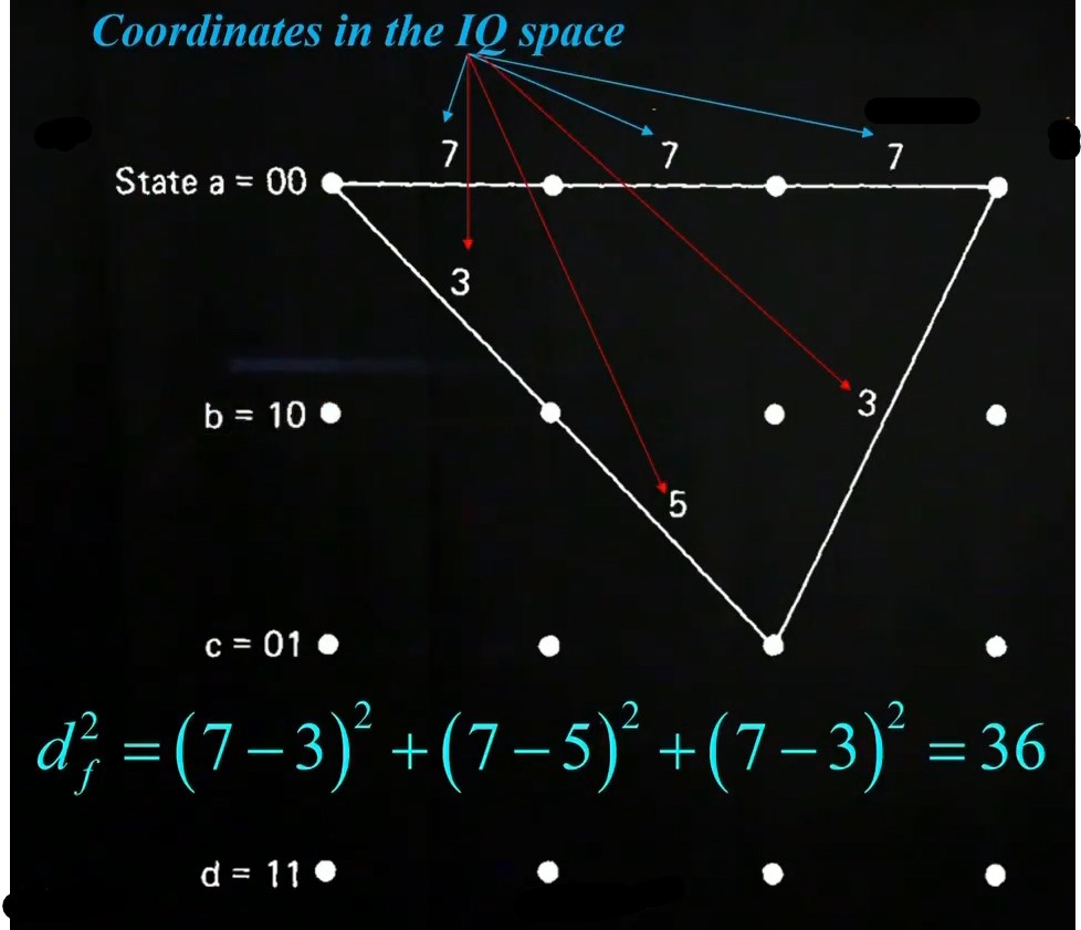
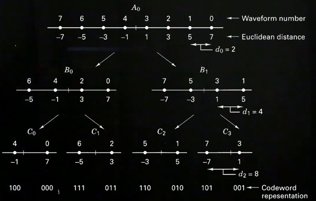


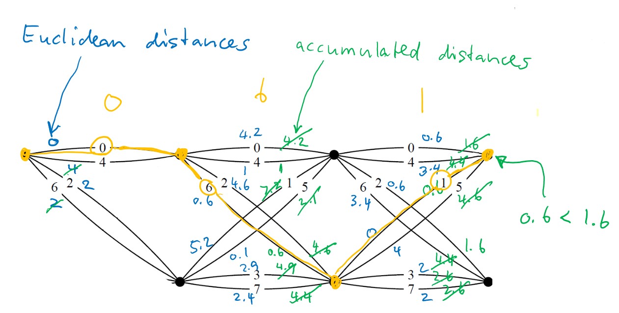


![-jNkdsinϕ
gg(ϕ) = w0 ⋅ 1 --e---------
-- 1 -|e- jk[dsin ϕ ]|
|| || |sin 1(N kd sin ϕ) |
|gg(ϕ )| = |w0| ⋅-||---2[1---------]||-
sin 2(kd sin ϕ)](main2_for_html345x.svg)


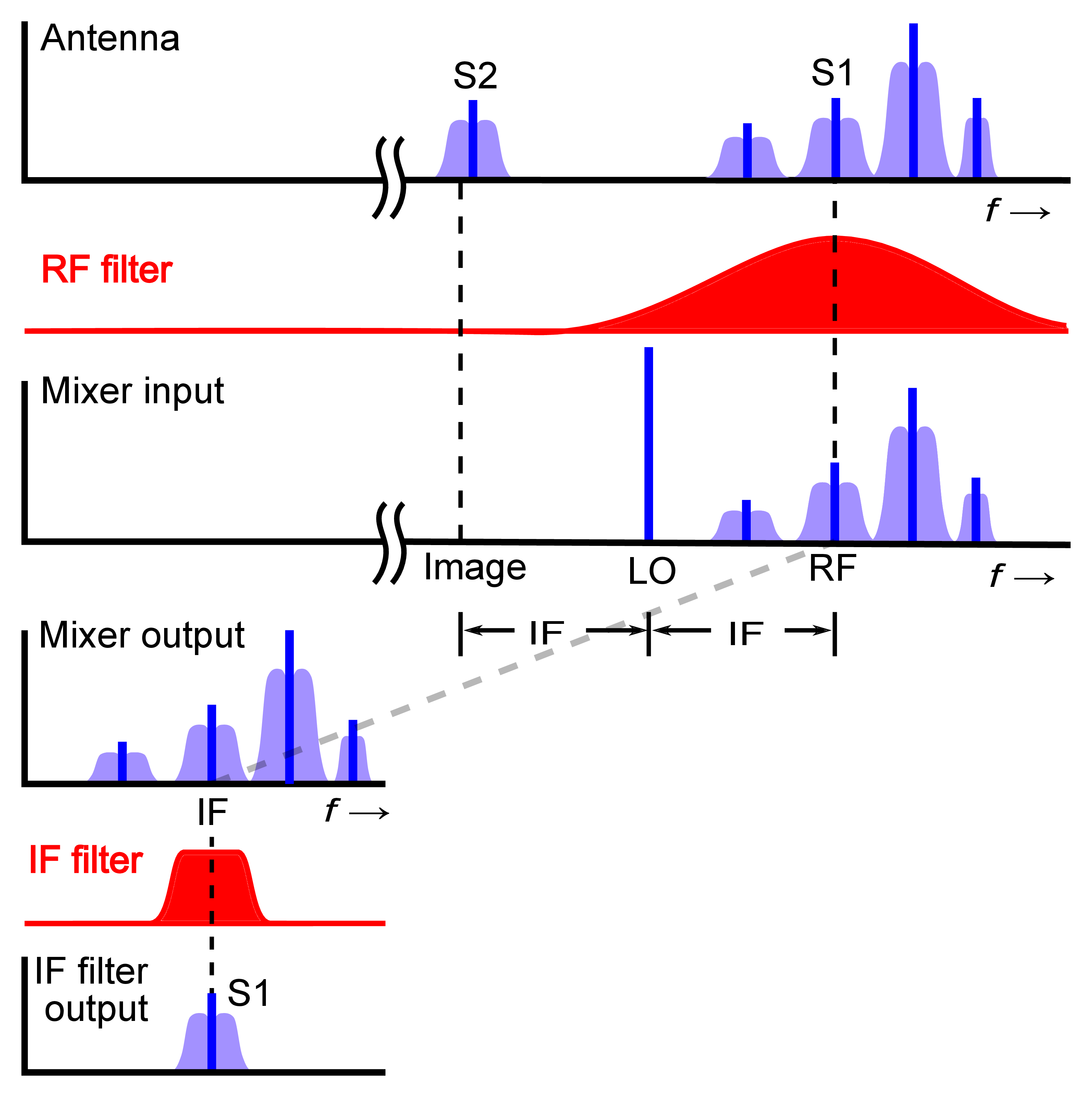


![E--
Zf = H = 120π ≈ 377[Ω]](main2_for_html393x.svg)


![( )
L [dB ] = 69.55 + 26.16 ⋅ log--f---- 13.82 ⋅ log hBS-- a(h ) + 44.9 - 6.55 log hBS- ⋅ log -d--
Hu M Hz m MS m km](main2_for_html399x.svg)


