Permanent magnets, explained with Maxwell's equations
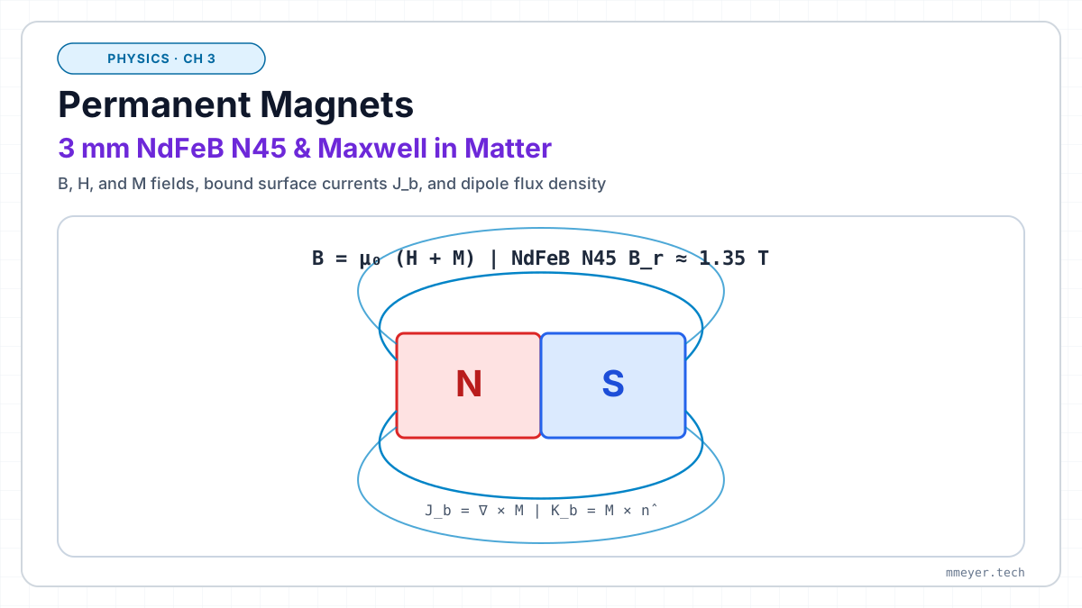
Chapter 2, Maxwell's equations explained, worked in vacuum. Here the equations go inside materials, which brings in D, H, polarization and magnetization. Then they are used to take apart a real product: a 3 mm NdFeB cube magnet of grade N45, line by line from its datasheet. All magnet fields are computed live from the exact formula for a uniformly magnetized cube.
Matter adds its own hidden charges and currents
Chapter 2 had only free charges and currents: electrons you put on a plate or push through a wire. Inside a material, every atom also reacts to the field:
Electric: polarization P
The field pulls each atom's electron cloud slightly away from its nucleus, or turns molecules that are already polar. Each one becomes a tiny electric dipole. P = dipole moment per volume (C/m²).
Inside a uniformly polarized piece, the + and − ends of neighbouring dipoles cancel. Where P ends at a surface, a layer of uncancelled bound charge remains:
Magnetic: magnetization M
Electrons spin and orbit their atoms, so each atom can act as a tiny current loop, a magnetic dipole. M = magnetic moment per volume (A/m).
Inside a uniformly magnetized piece, the loop currents of neighbouring atoms cancel. At the surface they do not, and a bound surface current flows around the piece:
Maxwell's equations from Chapter 2 stay exactly true, as long as you include these bound sources. But you rarely know them in advance. So two helper fields absorb them:
With D and H, only the free sources, the ones you control, remain visible:
| Law | Differential (in matter) | Integral (in matter) | Compared with vacuum |
|---|---|---|---|
| Gauss | ∇·D = ρf | ∯ D·dA = Qf,enc | E becomes D, and only free charge counts |
| Gauss for B | ∇·B = 0 | ∯ B·dA = 0 | unchanged: no magnetic charges, not even in matter |
| Faraday | ∇×E = −∂B/∂t | ∮ E·dl = −dΦB/dt | unchanged |
| Ampère-Maxwell | ∇×H = Jf + ∂D/∂t | ∮ H·dl = If,enc + dΦD/dt | B becomes H, and only free current counts |
To solve these you also need to know how the material responds, the constitutive relations. For linear materials, D = ε0εrE and B = μ0μrH. Examples: εr ≈ 4.4 for FR-4 board material and ≈ 80 for water; μr ≈ 1 for air and copper, hundreds to thousands for ferrites and electrical steel. A permanent magnet is not linear. It remembers its past (hysteresis). Near its working point, B ≈ Br + μ0μrecH with μrec ≈ 1.05. Sections 7 and 8 show where this comes from.
The plates carry a fixed free charge. In the slab, the molecules stretch into dipoles. Their ends form bound charge layers on the slab surfaces, − at the top and + at the bottom, which partly cancel the field. So E inside is εr times smaller. D is the same everywhere: its only sources are the free charges on the plates (∇·D = ρf), and the slab holds none. The difference between them is the polarization: D − ε0E = P.
Boundary conditions come straight from the integral forms
At the surface between two materials the fields can jump. The integral forms from Chapter 2 fix exactly how. Apply them to two tiny shapes that straddle the surface:
A flat pillbox gives the normal parts
Squeeze a closed box flat around the surface, so only its two lids count. ∯B·dA = 0 then gives Bn1 = Bn2: the normal part of B never jumps. In the same way, ∯D·dA = Qf gives Dn1 − Dn2 = σf.
A thin loop gives the tangential parts
Lay a narrow loop across the surface, so only its two long sides count. ∮H·dl = If gives Ht1 = Ht2 when no free surface current flows. ∮E·dl = −dΦ/dt → 0 gives Et1 = Et2.
Combine the two. Bn stays the same, while Bt = μHt scales with μ. So field lines bend at the surface, following tan θ2 / tan θ1 = μ2 / μ1. Here θ is measured from the surface normal.
Each line carries the same flux, so lines crowd together where B is strong. Turn μr up to steel values (1000 and more). In the steel the lines lie almost flat along the surface and are densely packed. Turn it around: any line that leaves steel into air leaves almost exactly perpendicular to the surface.
This is why magnets stick to steel, why transformer cores guide flux, and why steel shields work: steel gives B an easy path.
Huge numbers of aligned electron spins
Spin. Every electron is a tiny magnet with a moment of about one Bohr magneton, μB = 9.27·10⁻²⁴ A·m². In most atoms the electrons pair up with opposite spins and cancel.
Exchange. In iron, cobalt, nickel and some rare-earth compounds, a quantum-mechanical effect, the exchange interaction, makes neighbouring spins line up in parallel. It is far stronger than the magnetic force between them. In Nd₂Fe₁₄B about 2 μB per atom end up aligned. That gives the huge saturation polarization, Js = μ₀Ms ≈ 1.6 T at room temperature.
Temperature. Heat makes the spins wobble, which lowers the average alignment. At the Curie temperature (310 °C for this magnet) the order breaks down completely and the material becomes paramagnetic. Try the slider.
Anisotropy. The Nd₂Fe₁₄B crystal is tetragonal and has one strongly preferred "easy axis". Turning the magnetization away from it would take a field of about 7 T. The neodymium atoms supply this stiffness, and the iron atoms supply most of the moment. That is what makes the material magnetically hard: it keeps its direction.
Domains and grains. A sintered magnet is built from grains a few micrometres in size, with all their easy axes aligned during pressing. Before it is magnetized, each grain splits into domains that point up or down, and the net field is zero. In the factory, a strong field pulse sweeps the domain walls out (section 7).
Cartoon of a patch of atoms. Each arrow is one spin. The bar on the right is the net magnetization M, relative to its value at absolute zero.
No current, no charge, and still a field: M does it
A magnet lying on the table has no free current, and nothing changes in time. Maxwell's equations in matter shrink to three lines:
All of the field comes from M. Two exact and equivalent pictures turn this into something you can imagine:
Current model (Ampère)
Insert B = μ₀(H + M) into ∇×H = 0. You get ∇×B = μ₀∇×M = μ₀Jb, ordinary magnetostatics driven by bound currents. Inside a uniform magnet ∇×M = 0. On the side faces a surface current Kb = M×n̂ runs around the cube like the winding of a coil.
For the cube, |K| = M = Br/μ₀ = 1.07·10⁶ A/m. Over its 3 mm height that adds up to 3.2 kA, like a 3 mm coil with 3200 ampere-turns. No copper coil that small could carry this without burning. In the magnet the aligned spins "carry" it, without any loss.
B lines are closed loops that run through the magnet (∇·B = 0).
Charge model (Coulomb)
Insert B = μ₀(H + M) into ∇·B = 0. You get ∇·H = −∇·M = ρm. H then behaves like an electrostatic field with "magnetic charges" wherever M ends: σm = M·n̂, which is +M on the N face and −M on the S face.
Since ∇×H = 0, H is the gradient of a potential, so Coulomb-type integrals give it exactly. Every field on this page is computed that way. Inside the magnet, H points from N to S, against M. This is the demagnetizing field Hd = −N·M, and for a cube N = 1/3 by symmetry.
The "charges" are bookkeeping only. You can never isolate one (∯B·dA = 0).
Numbers for the 3 mm cube (Br = 1.35 T)
| Centre of the cube | H = −M/3, B = μ₀(H + M) = ⅔·Br | 0.90 T |
| Centre of the N face, just outside | formula below with z → 0 | 0.59 T |
| Middle of a side face, just outside | points backwards, from N towards S | 0.29 T |
| Magnetic moment | m = M·V = 1.07·10⁶ A/m · 27 mm³ | 0.029 A·m² |
| Far away (r ≫ 3 mm) | B = μ₀/4π · (3(m·r̂)r̂ − m)/r³ | dipole, falls as 1/r³ |
On the axis, at a distance z in front of the face of a cube with side a (charge model, exact):
The first term is the N face, which you see under a large solid angle when you are close. The second is the S face, further away, which subtracts. Right at the face the first term becomes π/2: you see half the field of an infinite charged plane, Br/2. Minus the S face, that gives 0.59 T. This is why the surface field is much smaller than Br.
A slice through the middle of the magnet
This is a vertical cut through the centre, with N on top. The colour shows the field strength on a log scale. Move the mouse over the picture to measure the field.
Move the mouse over the picture.
Now tick steel plate. The lines enter the steel perpendicularly (section 2). The steel acts like a mirror image of the magnet, so the cube behaves almost like a magnet twice as tall. Its internal field rises, and the densely packed lines at the contact pull. The pull per area is the Maxwell stress p = B²/2μ₀, about 4 bar at 1 T. Increase the gap and watch the force collapse.
Field lines around the cube, drag to rotate
25 field lines start on a grid across the middle of the magnet and follow B. Lines from near the edges make tight loops; lines from the centre swing far out. Every line closes through the magnet, and none starts or ends anywhere. The orange arrows (surface currents) circulate counter-clockwise when seen from the N side. Curl the fingers of your right hand along them and your thumb points to N.
Remanence and coercivity on the hysteresis loop
Imagine the magnet in a closed steel yoke with a coil around it, as in a factory measuring setup (a hysteresigraph). The yoke removes the demagnetizing field, so the coil sets the field inside the magnet directly. The graph shows the material's own polarization J = μ₀M and the flux density B = μ₀H + J.
- Virgin state. Each grain is split into up and down domains, so J = 0. Domain walls move easily, so a moderate field already magnetizes the grains.
- Saturation. Raise the field until every grain points up. Real NdFeB needs about 2400 kA/m for this (μ₀H ≈ 3 T), applied in the factory as a short pulse.
- Remanence Br. Switch the field off (H = 0). Nothing flips back, so J and B stay at Br = 1.35 T, the flux density that "remains". This is the datasheet's first big number.
- Normal coercivity bHc. Apply a reverse field. B drops along an almost straight line: the coil field cancels more and more of the polarization, while J itself stays at Br. Release the field before any grain flips and B springs back to Br. B alone would reach zero at Br/(μ₀μrec) ≈ 1020 kA/m. In N45 the first grains already flip at about 950 kA/m, so B reaches zero at about −950 kA/m (datasheet: 860–995). In grades with a higher iHc (SH, UH …), B passes zero while J is still completely intact.
- Intrinsic coercivity iHc. Push further. Near −950 kA/m, the "knee", grains start to flip. At iHc ≈ −1000 kA/m half of them have flipped and J = 0. This is irreversible: switching the field off leaves a weaker magnet. iHc measures how well the magnet resists being demagnetized.
Where a real magnet sits on its curve
A free magnet has no yoke. Its own H field (section 4) pushes the working point into the second quadrant of the loop, onto the demagnetization curve. Where exactly depends only on the shape. Since Hd = −N·M and B = μ₀(H + M), the working point lies on the load line:
Pc is the permeance coefficient. For the cube, N = 1/3 gives Pc = 2. Long magnets have a large Pc and work close to Br. Flat magnets have a small Pc and work deep down the curve, close to the knee.
Energy product (BH)max
The shaded rectangle is B·|H| at the working point. B·|H| times the magnet volume equals twice the energy stored in the magnet's external field. The largest possible rectangle is (BH)max, and the "45" in N45 refers to it. For a straight demagnetization curve, (BH)max = Br²/(4μ₀μrec) = 1.35²/(4·4π·10⁻⁷·1.05) = 345 kJ/m³ = 43.4 MGOe, which matches the datasheet's 342–358 kJ/m³. The cube works at 312 kJ/m³, about 90 % of the maximum.
Temperature: reversible and irreversible loss
Warming lowers Br (typically −0.12 %/K for NdFeB). This loss is reversible and comes back on cooling. Coercivity drops much faster, typically −0.6 %/K. Once the knee passes the working point, grains flip, and that loss is irreversible. Try the thin disc at 70 °C, cool it back down, and see that it stays weaker. The datasheet's 80 °C is a safe limit for common shapes. Above the Curie temperature (310 °C) all magnetization is gone.
Every line of the datasheet, explained and checked
| Parameter | Value | What it means, with a check |
|---|---|---|
| Artikel-ID, EAN | W-03-N 7640155438674 | The shop's article number and the EAN-13 barcode. The prefix 764 is registered with GS1 Switzerland. No physics here. |
| Werkstoff (material) | NdFeB | Neodymium-iron-boron, the compound Nd₂Fe₁₄B. Iron supplies the high magnetization, neodymium the strong easy axis, and boron stabilizes the crystal. It is the strongest permanent-magnet material in mass production. |
| Form, Seitenlänge, Toleranz | cube, 3 mm ± 0.1 mm | Volume 27 mm³. Within tolerance it ranges from 24.4 to 29.8 mm³, so moment and force can vary by about ±10 % from the tolerance alone. A cube has N = 1/3 and Pc = 2 (section 8). Magnetized through one pair of opposite faces. |
| Beschichtung (coating) | Ni-Cu-Ni | Three plated layers: nickel, copper, nickel, typically 10–20 µm in total. Bare NdFeB corrodes quickly, because the neodymium-rich grain boundaries oxidize and the magnet crumbles. The coating also adds a small gap between magnet and steel (section 10). |
| Herstellungsart (process) | gesintert (sintered) | The alloy is milled to a powder of single-crystal particles a few µm in size. The powder is pressed in a strong field so that all easy axes align (anisotropic magnet), sintered at about 1050–1100 °C, cut, ground, coated, and finally magnetized with a pulse field. Plastic-bonded magnets can be moulded into shape but are much weaker. |
| Magnetisierung (grade) | N45 | "45" means (BH)max ≈ 45 MGOe. "N" is the standard coercivity class, rated to 80 °C. The classes M, H, SH, UH and EH have higher iHc, usually from adding dysprosium or terbium, and survive higher temperatures. |
| Haftkraft (pull force) | ≈ 290 g = 2.84 N | The force needed to pull the magnet straight off a thick, flat steel plate. "290 g" means the weight of 290 g: 0.29 kg · 9.81 m/s² = 2.84 N. By the Maxwell stress p = B²/2μ₀, this takes an average of 0.89 T over the 9 mm² contact face. The ideal model (perfect steel, no gap) gives 5.3 N, and it drops to 2.84 N at an effective gap of only 0.2 mm (section 10). |
| Verschiebekraft (shear force) | ≈ 58 g = 0.569 N | The force needed to slide the magnet along the steel. The magnetic force acts perpendicular to the surface, so sideways only friction holds the magnet: 0.569 / 2.84 = 0.20, the friction coefficient. On a vertical steel wall the magnet therefore holds only about 1/5 of its pull force. |
| max. Einsatztemperatur | 80 °C | Maximum operating temperature. Above it, irreversible losses can start: coercivity falls by about 0.6 %/K until the knee reaches the working point (section 8). Flat shapes and opposing fields are more sensitive. |
| Farbe (colour) | silver | The colour of the nickel top layer. |
| Gewicht (weight) | 0.2052 g | Density = 0.2052 g / 0.027 cm³ = 7.6 g/cm³, typical for NdFeB. The magnet holds about 1400 times its own weight (290 g / 0.205 g). |
| Curie-Temperatur | 310 °C | Here the spin order collapses (section 3) and the material becomes paramagnetic. After cooling, the domains point randomly and the magnet is demagnetized. The microstructure may also be damaged. |
| Remanenz Br | 13 200–13 700 G 1.32–1.37 T | The flux density that remains inside after saturation, with H = 0 (closed circuit). 1 T = 10 000 G. Equal to Jr = μ₀Mr, so Mr ≈ 1.07·10⁶ A/m. It is not the surface field: a free cube has 0.90 T at its centre and 0.59 T at the centre of a face. It is lower than Js ≈ 1.6 T because the grains are not perfectly aligned and the grain-boundary phase is not magnetic. |
| Koerzitivfeldstärke bHc | 10.8–12.5 kOe 860–995 kA/m | Normal coercivity HcB: the reverse field at which B = 0. 1 Oe = 1000/4π A/m = 79.6 A/m. Reaching it is reversible, as long as you stay above the knee. The straight-line limit would be Br/(μ₀μrec) = 1023 kA/m. It comes out lower because the knee (iHc) is close. |
| Koerzitivfeldstärke iHc | ≥ 12 kOe ≥ 955 kA/m | Intrinsic coercivity HcJ: the reverse field at which the polarization J = 0, so half of the material has flipped. It measures resistance to demagnetization by heat, opposing fields or a flat shape. Always iHc ≥ bHc. |
| Energieprodukt (BH)max | 43–45 MGOe 342–358 kJ/m³ | Maximum energy product (section 8). 1 MGOe = 7.958 kJ/m³. Check: Br²/(4μ₀μrec) = 330–356 kJ/m³ for Br = 1.32–1.37 T. |
Unit converter
Field versus distance and force versus air gap
This is the field on the axis in front of the N face, on log-log scales. Close to the face the exact cube formula stays finite. Beyond about 1 cm the cube looks like a point dipole and B falls as 1/r³, so doubling the distance cuts the field to 1/8. At about 5 cm it has dropped to the strength of the Earth's field (≈ 48 µT).
The ideal model treats the steel as perfectly permeable and flat, which acts like a mirror magnet. The force is computed between the magnetic surface charges of the magnet and its image. At zero gap it gives 5.3 N. The datasheet's 2.84 N matches an effective gap of only 0.2 mm. Real steel has finite μ and saturates, and coating and roughness add gap. Small magnets lose force very quickly with distance, so paint, a label or a thin steel sheet cost much more.