TMR sensors, layer by layer: from a magnetic field to a number
A tunnel magnetoresistance (TMR) sensor turns a magnetic field into a digital number in seven steps. As in a network stack, each layer takes one quantity from the layer below, transforms it and hands a new quantity up: field → direction of a tiny magnet → tunnel current → resistance → voltage → digital code → angle or current. This page first shows the whole stack working at once, then opens every layer.
You need: magnetic fields and why iron is magnetic (chapter 3), Ampère's law (chapter 2) and quantum tunneling (chapter 9). The electronics of layer 6 is built from the devices of chapters 6–8. Next: chapter 11, another device that relies on tunneling.
Seven layers, like a network stack
In a network (digital track D1) every layer has one job and talks only to its neighbours: the physical layer moves bits, the data-link layer builds frames, and so on up to the application. A receiver unpacks the data from the bottom up. A sensor is a receiver for the physical world: the field enters at the bottom and climbs to the application on top. What each layer hands up is its "protocol data unit" (PDU), here a physical quantity.
| layer | receives | what happens | hands up |
|---|---|---|---|
| L1 field | a magnet, a current or the earth | the source produces a field at the chip | field B (mT) |
| L2 free layer | field B | a 2 nm magnetic film turns with the field | angle θ |
| L3 spin tunneling | angle θ | electrons tunnel more easily when both magnets are parallel | conductance G |
| L4 junction | conductance G | the film stack and the area set the resistance | resistance R (kΩ) |
| L5 bridge | four resistances | four junctions make a voltage and cancel temperature and offsets | voltage V (mV) |
| L6 signal chain | voltage V | amplifier and ADC turn volts into bits | digital code |
| L7 application | digital code | software computes what the user wants | angle (°), current (A) |
The analogy goes beyond the picture. As in a network, a layer can be replaced without touching the others: put a Hall plate in place of layers 2–4 (see Compare) and layers 5–7 stay the same, just as Wi-Fi can replace Ethernet underneath IP.
Move the magnet or the field and follow the "packet" up the stack. The right panel decodes it layer by layer, like a network analyser. Click a layer (or its button) for a closer look.
Where the field comes from, and how big it is
The input of the sensor is the magnetic flux density B, measured in tesla (T). In air it is tied to the field strength H by B = μ0H, so 1 mT corresponds to 796 A/m (and to 10 gauss). For scale: the earth's field is about 50 μT, a fridge magnet gives a few mT, the surface of a neodymium magnet about 0.5 T. Sensors meet three kinds of sources (chapter 3 and chapter 2):
- a permanent magnet on a rotating shaft (angle sensors). Far from it the field is that of a dipole and falls with the cube of the distance;
- a current in a wire (current sensors). Ampère's law gives circles around the wire, falling as 1/r;
- the earth (electronic compasses). Only its horizontal part, about 22 μT in central Europe, points north.
The magnet is a 6 mm × 2.5 mm NdFeB disc (Br = 1.3 T, magnetic moment m = 0.073 A·m²) treated as a point dipole. That is accurate once the distance exceeds the magnet's size; very close to it the real field is weaker than the dipole formula.
A tiny compass needle with a preferred axis
The sensing element is a ferromagnetic film only about 2 nm thick, the free layer. All its electron spins are aligned (chapter 3), so the whole film behaves like one compass needle: a magnetization vector of fixed length that can only rotate. It prefers to lie along an easy axis, set by the element's shape or crystal; the strength of that preference is the anisotropy field HK. An outside field H pulls the needle away from the easy axis. The Stoner–Wohlfarth model writes the energy, in units of the anisotropy energy, as a function of the magnetization angle θ:
θK is the direction of the easy axis, θH that of the field. The magnetization sits in a valley of e(θ), like a ball. The same film can be used in three ways:
- Field across the easy axis (linear sensor). One valley that moves smoothly: the component along the field is exactly cos θ = h for |h| ≤ 1. The response is linear, with no hysteresis.
- Field along the easy axis (memory). Two valleys. The ball stays in its valley until that valley disappears at |h| = 1, then it flips. The result is a square hysteresis loop, which is how MRAM stores a bit.
- Strong rotating field (angle sensor). The needle follows the field direction. A small lag remains, at most about 1/(2h) radians.
In memory mode the field is tilted 0.1° from the easy axis, as in any real experiment; otherwise the ball could balance forever on the top of the hill.
Electrons keep their spin while they tunnel
Every electron carries a spin, a built-in magnetic moment that points "up" or "down" along any chosen axis. In a ferromagnet the energy bands of the two spin directions are shifted against each other by the exchange splitting (about 1–2 eV in iron). At the Fermi energy, where conduction happens, there are therefore more states for one spin direction (the majority spins) than for the other (the minority spins). The spin polarization P measures the imbalance in the density of states D:
A magnetic tunnel junction is two ferromagnets separated by an insulator about 1 nm thick. Electrons cross it by quantum tunneling (chapter 9) and keep their spin on the way. Each electron needs a free state of the same spin on the other side, so each spin channel conducts in proportion to the product of the densities of states on both sides (Jullière, 1975). If the two magnetizations are parallel (P), majority meets majority and the current is large. If they are antiparallel (AP), majority meets minority and the current is small:
At an angle θ between the magnetizations, a spin that is "up" for the first magnet is, for the second, a quantum superposition: majority with probability cos²(θ/2), minority with probability sin²(θ/2). Adding the four channels gives a simple law. Note that it is the conductance G = 1/R, not the resistance, that varies with cos θ:
With P = 0.6 Jullière's formula gives 112.5 %. Real junctions do better than this simple model. Crystalline MgO lets mainly one symmetry of wave function through (called Δ1), and in Fe and CoFe(B) that symmetry is present at the Fermi energy almost only for majority spins. That raised room-temperature TMR from about 70 % with amorphous Al2O3 barriers to several hundred percent (record about 600 % in 2008). Sensors typically use 100–200 %.
Nine films, each a few nanometres thick
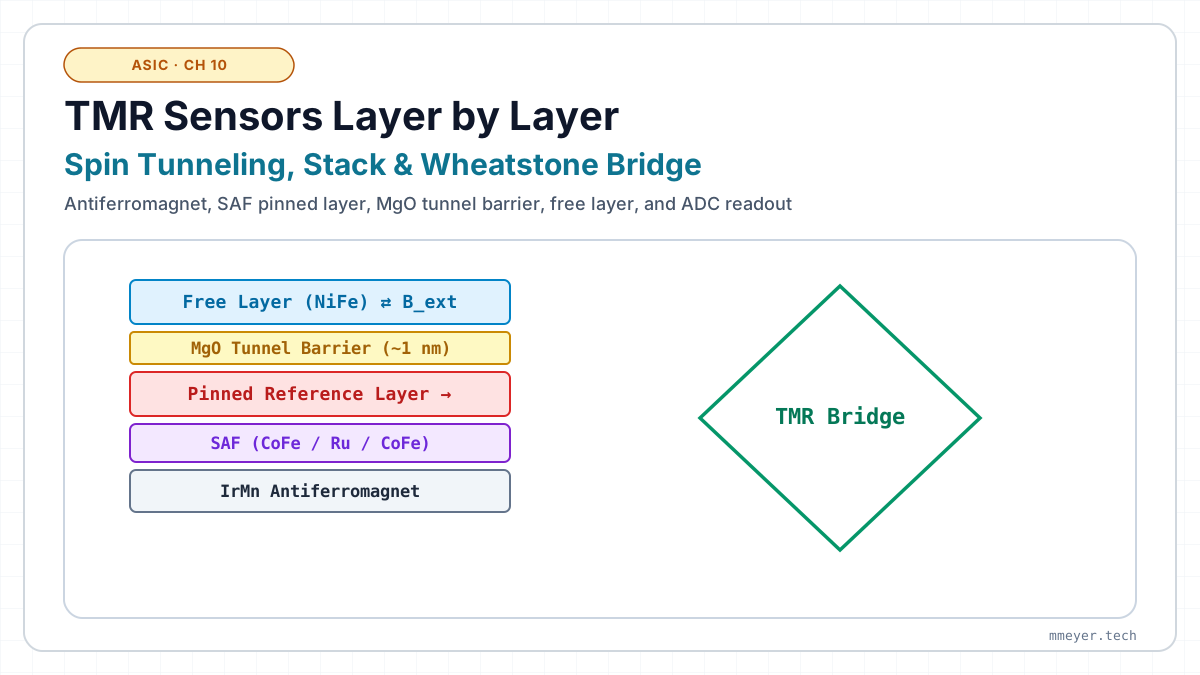
The real device is a stack of ultrathin films, sputtered onto the wafer and etched into pillars. Each film has a single job. Click a film in the picture to see its job.
- An antiferromagnet (IrMn or PtMn) pins the magnetization of the film on top of it by exchange bias. Its direction is set once, by cooling the wafer in a strong field.
- The pinned layer, a 0.85 nm ruthenium spacer and the reference layer form a synthetic antiferromagnet (SAF): through the Ru the two magnets couple antiparallel (RKKY coupling). The pair is very stiff and its stray fields almost cancel.
- The MgO barrier sets the resistance. Since tunneling falls off exponentially with thickness, the resistance-area product RA grows about ten-fold for every additional 0.25 nm.
- The free layer (CoFeB, sometimes with NiFe) turns with the field (layer 2), and a cap protects the stack.
The TMR also shrinks with the voltage across the barrier: hot electrons excite magnons and the spin filtering weakens. Sensors therefore connect many junctions in series in each bridge arm, so that every junction sees only some tens of millivolts. Series strings also average out noise and the variation between junctions.
Thicknesses and RA are typical values for CoFeB/MgO junctions; the formulas are fits that show the trends, not data of a specific product.
Four junctions turn resistance into a clean voltage
A single junction is a poor sensor on its own. Its resistance also changes with temperature, and it differs from chip to chip. A full Wheatstone bridge uses four junction strings. In two of them the reference layer is pinned one way, in the other two the opposite way (push-pull), so that a field raises the conductance of one pair exactly as much as it lowers that of the other. Everything that affects all four alike (temperature drift of R̄, supply noise, slow ageing) cancels, and the signal doubles. With R = R̄/(1 ± x) and x = P²h the output is exactly linear:
With Vb = 3.3 V, P² = 0.36 and HK = 5 mT the sensitivity is 72 mV per volt of supply per mT, and the output swings up to ±36 % of the supply. A silicon Hall plate gives about 0.1 mV/V/mT. What does not cancel: the TMR itself falls by about 0.1 % per kelvin, so the gain drifts. The electronics corrects that with a temperature sensor. Small mismatches between the four arms leave a small offset.
Amplify, digitize, and send it as bits
The bridge voltage is analog. An amplifier with gain G scales it to the input range VFS of an analog-to-digital converter (ADC), which outputs an N-bit number. The smallest step, one LSB, corresponds to a field step ΔB. Noise from the junctions (mostly 1/f noise at low frequency) and from the amplifier blurs the signal. Averaging Navg samples reduces random noise by √Navg, at the cost of speed. Too little gain wastes ADC resolution; too much gain clips strong fields. Here the sensor measures the earth's field while the device turns once every two seconds:
The codes at the bottom are what leaves the chip. A serial interface such as SPI or I²C packs them into frames. From here the sensor is literally part of a network stack: the bits travel over buses (AXI4-Lite on the processor side) and possibly over Ethernet and TCP (D1).
Angle, current, compass and memory
Angle sensors (steering wheels, motors, knobs) sit under a magnet on a rotating shaft. Two bridges with reference directions 90° apart give Vcos ∝ cos φ and Vsin ∝ sin φ, and the processor computes φ = atan2(Vsin, Vcos). Since the magnitude drops out, the result does not depend on the exact distance or temperature. It is sensitive to imperfections: an offset, unequal amplitudes or bridges not exactly 90° apart each cause a characteristic angle error. In the plot the circle becomes a shifted or squeezed ellipse.
- Current sensors measure the field of a conductor, B = μ0I/(2πr), without touching it: no shunt loss and galvanic isolation for free. Two sensors on opposite sides of the conductor see opposite fields; their difference doubles the signal and cancels homogeneous stray fields.
- Electronic compasses measure the 22 μT horizontal earth field along two or three axes and compute the heading with atan2, plus an accelerometer for tilt.
- MRAM stores a bit in the free layer: parallel = 0, antiparallel = 1 (layer 2, memory mode). It is read through the TMR and written by a current whose spin-polarized electrons exert a torque on the free layer (spin-transfer torque). It keeps its data without power like flash (chapter 11), but survives more than 1012 writes instead of about 105.
- Hard-disk read heads have used TMR since about 2005 to read magnetic bits only some tens of nanometres wide.
Hall, AMR, GMR and TMR: four ways to fill layers 2–4
| sensor | physical effect | signal | strengths and limits | typical use |
|---|---|---|---|---|
| Hall | the Lorentz force pushes the carriers to one side of a semiconductor plate | ≈ 0.1 mV/V/mT (silicon) | cheap and fully CMOS, works up to high fields; small signal, large offset | switches, current sensors, high-field angle sensors |
| AMR | resistance depends on the angle between current and magnetization (spin–orbit coupling) | ΔR/R ≈ 2–3 % | low noise and mature; the signal repeats every 180° | compasses, 180° angle sensors |
| GMR | spin-dependent scattering in metallic multilayers (Fert and Grünberg, Nobel prize 2007) | ΔR/R ≈ 10–20 % | large signal, low resistance | hard-disk heads 1997–2005, speed sensors |
| TMR | spin-dependent tunneling through MgO (this page) | ΔR/R ≈ 100–200 % (record ≈ 600 %) | largest signal, high resistance, so microwatt power; needs careful film growth | angle and current sensors, hard-disk heads, MRAM |
The stack on one page
| layer | key idea | formula |
|---|---|---|
| L1 field | dipole falls as 1/d³, wire as 1/r | B = μ0I/(2πr) |
| L2 free layer | a single rotating magnetization in an energy valley | e = sin²(θ−θK) − 2h cos(θ−θH) |
| L3 spin tunneling | spin is conserved while tunneling | G = Ḡ(1 + P²cos θ), TMR = 2P²/(1−P²) |
| L4 junction | exponential in barrier thickness, weaker at high bias | R = RA/A |
| L5 bridge | push-pull cancels common drifts, exactly linear | V = VbP²h |
| L6 signal chain | gain trades range against resolution | ΔB = VFS/(2N·G·S·Vb) |
| L7 application | ratios such as atan2 cancel common errors | φ = atan2(Vsin, Vcos) |
Where next? Chapter 11 stores data with tunneling electrons as well, as charge on a floating gate instead of in a magnet. Back to the learning path.
Every term on this page
| TMR | tunnel magnetoresistance: (RAP − RP)/RP |
| MTJ | magnetic tunnel junction: ferromagnet / thin insulator / ferromagnet |
| B, H, μ0 | flux density (T), field strength (A/m), B = μ0H in air, μ0 = 4π·10⁻⁷ T·m/A |
| dipole moment m | strength of a small magnet (A·m²); its field falls as 1/d³ |
| free layer, reference layer | the magnet that turns with the field; the one that is held fixed |
| easy axis, anisotropy field HK | preferred direction of the magnetization; the field needed to pull it fully away |
| Stoner–Wohlfarth model | a magnet as one rotating vector in an energy landscape |
| hysteresis, switching field | the state depends on the history; the field at which the old state disappears |
| spin, majority / minority | the electron's magnetic moment; the more / less numerous spin direction at EF |
| exchange splitting | energy shift between the spin-up and spin-down bands of a ferromagnet |
| spin polarization P | imbalance of the two spin densities of states at the Fermi energy |
| Jullière model | TMR from the spin polarizations: 2P1P2/(1 − P1P2) |
| Δ1 filtering | crystalline MgO transmits mainly one wave-function symmetry, which is almost fully spin-polarized |
| RA product | resistance × area, the barrier's property independent of pillar size |
| exchange bias, antiferromagnet | pinning of a ferromagnet by an adjacent antiferromagnet (IrMn, PtMn) |
| SAF, RKKY coupling | two magnets coupled antiparallel through a thin Ru layer |
| Wheatstone bridge, push-pull | four resistors giving a difference voltage; arms that change in opposite directions |
| sensitivity S | output per supply voltage per field, mV/V/mT |
| ADC, LSB, gain | analog-to-digital converter; its smallest step; amplification before it |
| 1/f noise, averaging | noise rising at low frequency; combining samples to reduce random noise |
| atan2 | the angle of a point (x, y) over the full 360° |
| MRAM, spin-transfer torque | magnetic memory; switching a magnet with a spin-polarized current |
| Hall, AMR, GMR | other magnetic sensor effects, compared above |